Provable Acceleration of Nesterov's Momentum for Deep ReLU Networks

§ 01 · Origins

A stubborn open question

Nesterov's momentum buys gradient descent a factor of \(\sqrt{\kappa}\) on smooth, strongly convex problems — a textbook result from Nesterov (2018). For neural networks, it is long-standing folklore that momentum helps (Sutskever et al., 2013). Folklore is not theory, and theory has been stubborn. Three specific obstructions have kept the field off-balance:

Most neural-network convergence proofs lean on the Polyak–Łojasiewicz (PL) condition (Karimi et al., 2016). Under PL, gradient descent is linear — and Yue et al. (2022) showed it is rate-optimal. PL alone gives momentum nothing to improve.
Known accelerated rates under PL-like conditions either assume extra structure that is hard to verify on neural nets (Wang et al., 2022's \(\lambda^{\star}\)-average), or only cover shallow / linear networks (Wang et al., 2021; Liu et al., 2022).
In a non-convex setting, just constructing a working Lyapunov function for Nesterov's iteration is delicate. There can be many global minima, so the classical estimating-sequence argument breaks.

The question, one sentence: is there a realistic regulatory condition on the loss of a deep network under which Nesterov's momentum provably accelerates?

§ 02 · The Idea

The partition model

The paper refuses the false dichotomy between "fully strongly convex" and "only PL". What if the parameters split into two pieces, and only one piece behaves nicely? Formally, we minimize

\[ \min_{\mathbf{x}\in\mathbb{R}^{d_1},\,\mathbf{u}\in\mathbb{R}^{d_2}} f(\mathbf{x}, \mathbf{u}) \]

where \(f\) is smooth and \(\mu\)-strongly convex in \(\mathbf{x}\) alone, with mild Lipschitz-in-\(\mathbf{u}\) control on the model and gradient, plus a "universal optimality" assumption — the minimum over \(\mathbf{x}\) for any fixed \(\mathbf{u}\) in a small neighborhood around initialization already hits the global minimum. Crucially, \(f\) is never required to be convex or even smooth in \(\mathbf{u}\).

Fig. 1 The partition model. Gradient methods are agnostic to this partition — they never see it. But the analysis uses the structure to bound how updates on \(\mathbf{u}\) perturb progress on \(\mathbf{x}\).

Assumption	What it says
A1. Partial strong convexity	\(f\) is \(\mu\)-strongly convex in \(\mathbf{x}\) for every fixed \(\mathbf{u}\) near \(\mathbf{u}_0\).
A2. Partial smoothness	\(f\) is \(L_1\)-smooth in \(\mathbf{x}\).
A3. Outer-loss smoothness	\(f = g\circ h\) with \(g\) being \(L_2\)-smooth (MSE, logistic, …).
A4. \(h\) is \(G_1\)-Lipschitz in \(\mathbf{u}\)	Model output changes slowly with \(\mathbf{u}\).
A5. \(\nabla_{\mathbf{x}} f\) is \(G_2\)-Lipschitz in \(\mathbf{u}\)	The \(\mathbf{x}\)-gradient is stable under \(\mathbf{u}\) perturbations.
A6. Universal optimality	\(\min_{\mathbf{x}} f(\mathbf{x},\mathbf{u}) = f^{\star}\) for every \(\mathbf{u}\) in a small neighborhood around initialization — fully optimizing \(\mathbf{x}\) at any such \(\mathbf{u}\) already reaches the global min.

These assumptions sit strictly between smooth-plus-strongly-convex (which implies them) and PL (which they imply). Proof techniques for this class do real work beyond the PL literature.

Most of the signal in the gradient flows through \(\mathbf{x}\). The wild side of the network is not dead — it is just quieter than the nice side.

§ 03 · The Theorem

Acceleration, deterministically

Run Nesterov's momentum with constant step \(\eta\) and momentum parameter \(\beta\), with no awareness of the partition:

\[ \begin{aligned} (\mathbf{x}_{k+1}, \mathbf{u}_{k+1}) &= (\mathbf{y}_k, \mathbf{v}_k) - \eta\,\nabla f(\mathbf{y}_k, \mathbf{v}_k), \\ (\mathbf{y}_{k+1}, \mathbf{v}_{k+1}) &= (\mathbf{x}_{k+1}, \mathbf{u}_{k+1}) + \beta\bigl((\mathbf{x}_{k+1}, \mathbf{u}_{k+1}) - (\mathbf{x}_k, \mathbf{u}_k)\bigr). \end{aligned} \]

Theorem 7 · Informal

Under Assumptions A1–A6 (more details in the paper), with \(G_1, G_2\) sufficiently small and \(R_{\mathbf{x}}, R_{\mathbf{u}}\) sufficiently large, choose \(\eta = \Theta(1/L_1)\) and \(\beta = \tfrac{4\sqrt{\kappa}-\sqrt{c}}{4\sqrt{\kappa}+7\sqrt{c}}\). Then

\[ f(\mathbf{x}_k, \mathbf{u}_k) - f^{\star} \;\leq\; 2\bigl(1 - \tfrac{c}{4\sqrt{\kappa}}\bigr)^{k}\bigl(f(\mathbf{x}_0, \mathbf{u}_0) - f^{\star}\bigr). \]

Compared with gradient descent under the same assumptions, which converges at \(1 - \Theta(1/\kappa)\) (Theorem 6), momentum earns the familiar factor of \(\sqrt{\kappa}\).

\(\kappa\) = 100

GD — \((1 - 1/\kappa)^k\) Nesterov — \((1 - 1/\sqrt{\kappa})^k\) target accuracy \(\varepsilon = 10^{-2}\)

This does not correspond to an actual experiment, but is shown for illustration purposes only. Error is plotted on a log scale — standard convention, smaller is better. Both methods start at error 1. The dashed line is a target accuracy of 10⁻². The two dots mark the iteration at which each method hits that target. At \(\kappa = 100\), GD takes roughly ten times as long as Nesterov; drag the slider to see how the gap scales with \(\sqrt{\kappa}\).

Read the fine print

The theorem is conditional. For the bound to apply, the paper requires

\[ G_1^4 \lesssim \tfrac{\mu^2}{L_2(L_2+1)^2}\bigl(\tfrac{1-\beta}{1+\beta}\bigr)^3, \qquad G_1^2 G_2^2 \lesssim \tfrac{\mu^3}{L_2(L_2+1)\sqrt{\kappa}}\bigl(\tfrac{1-\beta}{1+\beta}\bigr)^2, \]

plus lower bounds on \(R_{\mathbf{x}}, R_{\mathbf{u}}\). Translation: the non-convex part of the problem has to be a sufficiently mild perturbation of the nice part. When \(G_1, G_2\) are not small, the guarantee breaks — and, as the experiments below show, so does the empirical advantage.

§ 04 · Craft

Two difficulties, two lemmas

Under strong convexity, the standard Bansal–Gupta (2019) Lyapunov function uses the global minimizer \(\mathbf{w}^{\star}\) as a reference point. In the partition model, two things break at once.

Difficulty 1. \(f\) can have many global minima, so there is no canonical anchor. The paper's fix: re-anchor to \(\mathbf{x}^{\star}(\mathbf{u}_k) = \arg\min_{\mathbf{x}} f(\mathbf{x},\mathbf{u}_k)\) — a moving reference point. This requires controlling how fast the anchor slides:

Lemma 8 (Moving minimum). \(\|\mathbf{x}^{\star}(\mathbf{u}_1) - \mathbf{x}^{\star}(\mathbf{u}_2)\|_2 \leq \tfrac{G_2}{\mu}\|\mathbf{u}_1 - \mathbf{u}_2\|_2\)

Fig. 2 As \(\mathbf{u}\) drifts during Nesterov's iteration, the reference minimizer \(\mathbf{x}^{\star}(\mathbf{u})\) slides along with it. Lemma 8 caps the slide by \(G_2/\mu\) — which is why the paper needs \(G_2\) small.

Difficulty 2. Nesterov's update evaluates the gradient at the extrapolated point \((\mathbf{y}_k, \mathbf{v}_k)\), not at \((\mathbf{x}_k, \mathbf{u}_k)\). Standard bounds of the form \(\|\nabla f\|^2 \leq 2L(f - f^{\star})\) connect to the optimality gap at the point where the gradient is taken — but we only know the gap at \((\mathbf{x}_k, \mathbf{u}_k)\). The fix is a gradient-dominance lemma:

Lemma 9 (Gradient dominance). \(\|\nabla_{\mathbf{u}} f(\mathbf{x}, \mathbf{u})\|_2^2 \leq \tfrac{G_1^2 L_2}{\mu}\,\|\nabla_{\mathbf{x}} f(\mathbf{x}, \mathbf{u})\|_2^2.\)

The gradient on the wild side is dominated by the gradient on the nice side. Together with a carefully chosen Lyapunov function

\[ \phi_k = f(\mathbf{x}_k, \mathbf{u}_k) - f^{\star} + \mathcal{Q}_1 \|\mathbf{z}_k - \mathbf{x}^{\star}_{k-1}\|_2^2 + \tfrac{\eta}{8}\|\nabla_{\mathbf{x}} f(\mathbf{y}_{k-1}, \mathbf{v}_{k-1})\|_2^2, \]

this is enough to recover the \(1 - \Theta(1/\sqrt{\kappa})\) rate. The third term absorbs the errors from updating \(\mathbf{u}\) — a concern standard proofs never have to worry about.

§ 05 · In the Wild

Where the partition actually shows up

Realization 1: additive models. With \(h(\mathbf{x}, \mathbf{u}) = \mathbf{A}_1 \mathbf{x} + \sigma(\mathbf{A}_2 \mathbf{u})\) under MSE loss, the objective is non-convex (because of \(\sigma\), which can be ReLU) and potentially non-smooth — yet the assumptions are satisfied with \(\mu = \sigma_{\min}(\mathbf{A}_1)^2\), \(L_1 = \sigma_{\max}(\mathbf{A}_1)^2\), \(G_1 = B\,\sigma_{\max}(\mathbf{A}_2)\), and \(G_2 = B\,\sigma_{\max}(\mathbf{A}_1)\sigma_{\max}(\mathbf{A}_2)\) for a \(B\)-Lipschitz \(\sigma\). The non-convexity is controlled by \(\sigma_{\max}(\mathbf{A}_2)\) — a single knob.

Realization 2: deep fully-connected ReLU networks. This is the headline. Partition the parameters into \(\mathbf{x} = \mathrm{vec}(\mathbf{W}_{\Lambda})\) (last-layer weights — with some complications for handling the null space induced by over-parameterization; see the paper for details) and \(\mathbf{u} = (\mathrm{vec}(\mathbf{W}_1), \dots, \mathrm{vec}(\mathbf{W}_{\Lambda-1}))\) (all earlier layers). MSE loss is strongly convex in \(\mathbf{x}\) at fixed \(\mathbf{u}\) provided the penultimate-layer feature matrix is full-rank — which holds at standard Gaussian initialization under sufficient width.

Theorem 15 · Informal

For a \(\Lambda\)-layer ReLU network with standard Gaussian initialization, if intermediate widths are \(\Theta(m)\) and the penultimate width satisfies \(d_{\Lambda-1} = \Omega(n^{4.5}\max\{n, d_0^2\})\), then Nesterov's momentum trained on MSE loss satisfies

\[ \mathcal{L}(\boldsymbol{\theta}_k) \leq 2\bigl(1 - \tfrac{c}{4\sqrt{\kappa}}\bigr)^k \mathcal{L}(\boldsymbol{\theta}_0), \qquad \kappa = \tfrac{2L_1}{\alpha_0^2}, \]

with high probability over initialization. To our knowledge, this is the first accelerated convergence rate proven for a non-trivial (i.e., non-shallow, non-linear) neural-network architecture.

What this is, and is not

The width requirement \(\Omega(n^{4.5}\max\{n, d_0^2\})\) — which simplifies to \(\Omega(n^{5.5})\) when \(d_0 \leq n\) — is a sufficient condition for the proof. Like much of the NTK literature, it is not a claim about what works in practice. The same caveat applies to the "sufficiently small \(G_1, G_2\)" conditions: the result tells you when acceleration is provable, not that your favourite over-parameterized network clears the bar. Empirically, networks seem to benefit from momentum well outside this regime; proving that requires new ideas.

§ 06 · Evidence

Three regimes, one knob

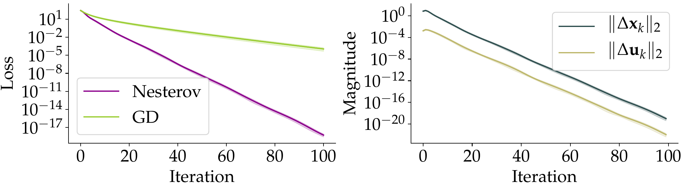
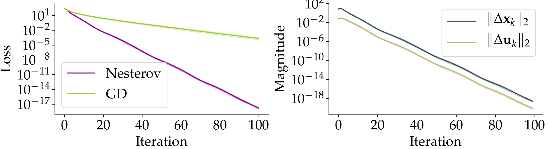
The cleanest empirical test is the additive model with \(h(\mathbf{x}, \mathbf{u}) = \mathbf{A}_1\mathbf{x} + \sigma(\mathbf{A}_2\mathbf{u})\), ReLU nonlinearity, MSE loss. Both \(G_1\) and \(G_2\) scale with \(\sigma_{\max}(\mathbf{A}_2)\), so sweeping that single knob traces out in-theory vs out-of-theory regimes. Left columns: loss vs iterations (mean over 10 trials; shaded = std). Right columns: evolution of \(\|\Delta \mathbf{x}_k\|_2\) vs \(\|\Delta \mathbf{u}_k\|_2\).

Experiment 1: sigma_max(A_2) = 0.01 — **Fig. 3a · In-regime** \(\sigma_{\max}(\mathbf{A}_2) = 0.01\). Deep in the regime of the theorem. Nesterov (purple) clearly accelerates over GD (green). Std bands are tiny; per-trial behaviour is reproducible. Right: \(\|\Delta \mathbf{x}_k\|_2 \gg \|\Delta \mathbf{u}_k\|_2\), and both decay linearly — matching the prediction of Lemma 10.

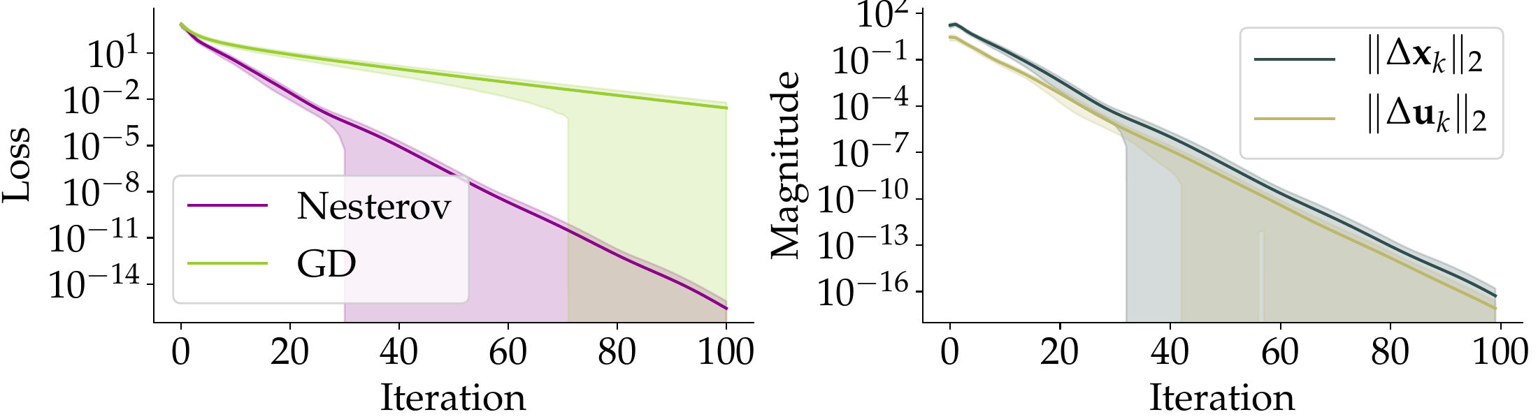
Experiment 2: sigma_max(A_2) = 0.3 — **Fig. 3b · On the edge** \(\sigma_{\max}(\mathbf{A}_2) = 0.3\). Nesterov still accelerates, but the update on \(\mathbf{u}\) is closer in magnitude to the update on \(\mathbf{x}\). The dashed line for \(\|\Delta \mathbf{u}_k\|\) visibly climbs relative to \(\|\Delta \mathbf{x}_k\|\), as the gradient-dominance bound predicts.

Experiment 3: sigma_max(A_2) = 5 — **Fig. 3c · Outside the theorem** \(\sigma_{\max}(\mathbf{A}_2) = 5\). Shaded bands widen: initialization now matters, and the Nesterov advantage becomes fragile. Exactly what the conditional nature of the theorem predicts — the bound is telling the truth in both directions.

The last plot is, in a way, more informative than the first. It shows what fails when the partition-model assumptions are violated.

The theorem does not predict that momentum stops working outside its regime; it predicts that the tight acceleration guarantee no longer holds and outcome variance grows. Both predictions are visible above.

§ 07 · Ledger

What is proven, what is open

✓ Proven here

GD gets rate \(1 - \Theta(1/\kappa)\) on the partition model (Thm 6).
Nesterov's momentum gets \(1 - \Theta(1/\sqrt{\kappa})\) on the partition model (Thm 7), under small-\(G_1,G_2\) conditions.
Additive models satisfy the assumptions; acceleration holds when the non-convex amplitude \(\sigma_{\max}(\mathbf{A}_2)\) is small enough (Thm 13).
Deep FC ReLU nets trained with MSE under standard Gaussian init satisfy the assumptions at width \(\Omega(n^{4.5}\max\{n, d_0^2\})\) (Lemma 14).
Nesterov's rate on deep FC ReLU nets is \(1 - \Theta(1/\sqrt{\kappa})\) — the first such result for a non-trivial architecture (Thm 15).

↪ Open / next

Removing the universal-optimality assumption (A6) — what if fully optimizing \(\mathbf{x}\) does not reach \(f^{\star}\)?
Beyond fully-connected ReLU — do CNNs and ResNets admit a similar partition?
Connecting to neural-network pruning — does the Lottery Ticket Hypothesis preserve partition-model structure?
Tightening the width requirement — is \(n^{4.5}\) the right exponent?

§ 08 · Final notes

Why we wrote this paper

Acceleration is one of the great stories of convex optimization — since Nesterov's 1983 result, the \(\sqrt{\kappa}\) speedup has been celebrated, generalized, and taught as canonical. For non-convex optimization, the story has been a persistent mystery. Neural-network trainers empirically reach for momentum; theorists have struggled to say why.

Two prior negative results explain the difficulty. Under the Polyak–Łojasiewicz condition — the standard scaffolding for non-convex convergence proofs in deep learning — Yue et al. (2022) showed that gradient descent is already rate-optimal; no \(\sqrt{\kappa}\) left for momentum. For the Heavy Ball method, Goujaud et al. (2023) proved it cannot accelerate even on smooth and strongly convex functions.

Our hope is to carry the machinery of convex-optimization theory an ε-step beyond the class of convex functions — and to keep the speedup intact on the way out.

The partition model sits strictly between PL and full strong convexity: strong enough to support an accelerated Lyapunov argument, weak enough to cover deep ReLU training with MSE. To our reading, this is the first time the convex toolbox has been extended to a non-shallow, non-linear neural-network setting while keeping the accelerated rate. One step, not a mile.

Caveats, one more time

Everything above is for full-batch gradients, fully-connected ReLU networks, and MSE loss, under standard Gaussian initialization with width \(\Omega(n^{5.5})\) (assuming \(d_0 \leq n\)). We do not claim the result applies to practical ResNet training, nor that Nesterov is empirically the best optimizer in any given application. What we claim is that theory has caught up to a well-known empirical phenomenon in one clean regime, and that the proof technique generalizes further than it may initially appear.

Cite as

F. Liao and A. Kyrillidis. Provable Accelerated Convergence of Nesterov's Momentum for Deep ReLU Neural Networks. International Conference on Algorithmic Learning Theory (ALT), PMLR vol. 237, 2024. [PDF]

When does Nesterov's momentum actually accelerate deep learning?