(Blog post by Junhyung Lyle Kim - see also here)

This blog post is about my recent work on quantum state tomography using (accelerated) non-convex programming.¹ Our manuscript is on arXiv. This is a joint work with my advisor Prof. Tasos Kyrillidis at Rice University, Dr. Amir Kalev at USC, and Dr. Georgios Kollias and Dr. Ken Wei at IBM Quantum.

Introduction

Quantum state tomography (QST) is one of the main procedures to identify the nature of imperfections in quantum processing unit (QPU) implementation. High-level procedure is to measure the quantum system, estimate the density matrix using the measured data, and analyze the “fit” between the estimated density matrix and the true density matrix.

QST is generally not scalable due to two bottlenecks: \(i)\) large data has to be collected to perform tomography; and \(ii)\) the space of density matrices grows exponentially, from which the one that is consistent with the data has to be found.

To address the first bottleneck, prior information is often assumed and leveraged to reduce the number of data required. For example, in compressed sensing QST, ^{2 3} it assumes that the density matrix is of low-rank. Similarly, in neural network QST, the wavefunctions are assumed to be real and positive. ^{4 5 6}

To give a concrete example, in the figure below, real (top) and imaginary (bottom) parts of four different states are shown: \(i)\) \(\texttt{GHZ}\) state, \(ii)\) \(\texttt{GHZminus}\) state, \(iii)\) \(\texttt{Hadamard}\) state, and \(iv)\) \(\texttt{Random}\) state; for the mathematical description of the above states, refer to our paper. ¹ As can be seen, for \(\texttt{GHZ}\) and \(\texttt{GHZminus}\) states, only four corners of the real parts have non-zero entries. Therefore, the density matrices of these states are both of low-rank and sparse. If these kinds of “structures” are smartly leveraged, one can sometimes confine the search space of density matrices greatly, leading to less number of measurements required for successful tomography results.

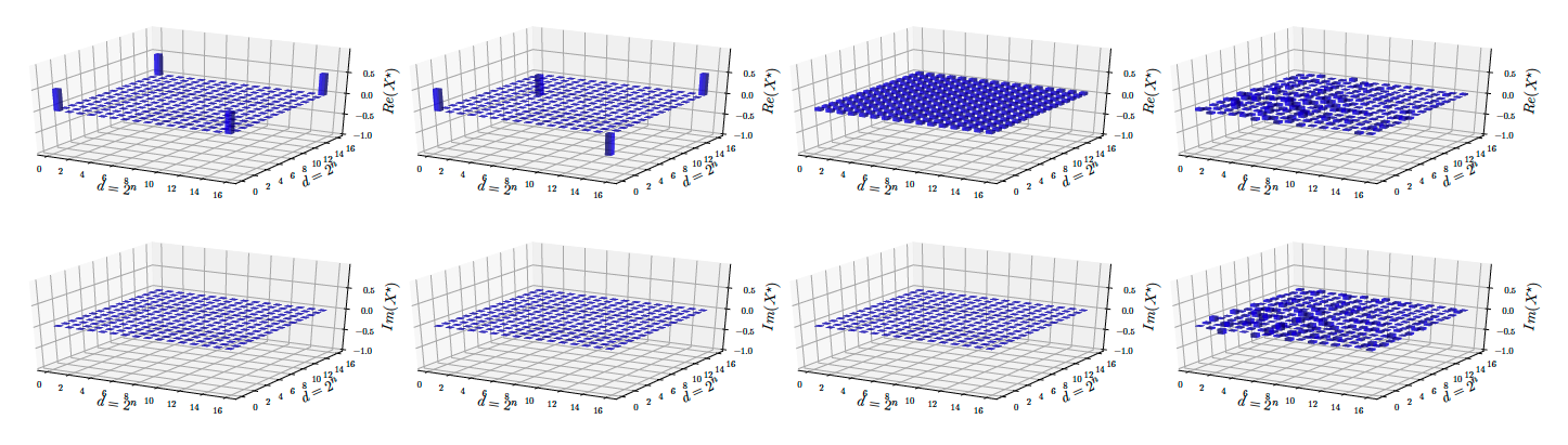
From left to right: GHZ, GHZminus, Hadamard, and Random states. All states are in 4-qubit system.

With regards to the second bottleneck, variants of gradient descent convex solvers were proposed under synthetic scenarios. ^{7 8 9 10} However, due to the exponentially increasing space of density matrices, these methods often can be only applied to relatively small system, on top of relying on special-purpose hardwares and proper distributed system designs.¹¹

On the contrary, non-convex optimization methods can perform much faster. It was recently shown that one can formulate compressed sensing QST as a non-convex problem,¹² which can be solved with rigorous convergence guarantees, allowing density matrix estimation in a large system. A relevant result can be seen in the Results section below, where we compare our proposed (accelerated) non-convex method with convex methods from \(\texttt{Qiskit}\).

In this work, we consider the setup where \(n\)-qubit state is close to a pure state, thus its density matrix is of low-rank. We introduce an accelerated non-convex algorithm with provable gaurantees, which we call \(\texttt{MiFGD}\), short for “\(\texttt{M}\)omentum \(\texttt{i}\)nspired \(\texttt{F}\)actored \(\texttt{G}\)radient \(\texttt{D}\)escent.”

Problem setup

We consider the reconstruction of a low-rank density matrix \(\rho^\star \in \mathbb{C}^{d \times d}\) on a \(n\)-qubit Hilbert space, where \(d=2^n\), through the following \(\ell_2\)-norm reconstruction objective:

\begin{align} \label{eq:objective} \tag{1} \min_{\rho \in \mathbb{C}^{d \times d}} \quad & f(\rho) := \tfrac{1}{2} ||\mathcal{A}(\rho) - y||_2^2 \quad \text{subject to} \quad \rho \succeq 0, ~\texttt{rank}(\rho) \leq r. \end{align}

Here, \(y \in \mathbb{R}^m\) is the measured data through quantum computer or simulation, and \(\mathcal{A}(\cdot): \mathbb{C}^{d \times d} \rightarrow \mathbb{R}^m\) is the linear sensing map. The sensing map relates the density matrix \(\rho\) to the measurements through Born rule: \(\left( \mathcal{A}(\rho) \right)_i = \text{Tr}(A_i \rho),\) where \(A_i \in \mathbb{C}^{d \times d},~i=1, \dots, m\) are the sensing matrices. From the objective function above, we see two constraints: \(i)\) the density matrix \(\rho\) is a positive semidefinite matrix (which is a convex constraint), and \(ii)\) the rank of the density matrix is less than \(r\) (which is a non-convex constraint).

As mentioned earlier, we focus on compressed sensing quantum state tomography setting, where the number of measured data \(m\) is much smaller than the problem dimension \(O(d^2)\). Compressed sensing is a powerful optimization framework developed mainly by Emmanuel Candès, Justin Romberg, Terence Tao and David Donoho, and requires the following pivotal assumption on the sensing matrix \(\mathcal{A}(\cdot)\), namely the Restricted Isometry Property (RIP) (on \(\texttt{rank}\)-\(r\) matrices): ¹³

\begin{align} \label{eq:rip} \tag{2} (1 - \delta_r) \cdot || X ||_F^2 \leq || \mathcal{A}(X) ||_2^2 \leq (1 + \delta_r) \cdot ||X||_F^2. \end{align}

Intuitively, the above RIP assumption states that the sensing matrices \(\mathcal{A}(\cdot)\) only “marginally” changes the norm of the matrix \(X\).

Going back to the main optimization problem in Eq. \eqref{eq:objective}, instead of solving it as is, we propose to solve a factorized version of it, following recent work ¹²: \begin{align} \label{eq:factored-obj} \tag{3} \min_{U \in \mathbb{C}^{d \times r}} f(UU^\dagger) := \tfrac{1}{2} || \mathcal{A} (UU^\dagger) - y ||_2^2, \end{align} where \(U^\dagger\) denotes the adjoint of \(U\). The motivation is rather clear: in the original objective function in Eq. \eqref{eq:objective}, the density matrix \(\rho\) is represented as a \(d \times d\) Hermitian matrix, and due to the (non-convex) \(\texttt{rank}(\cdot)\) constraint, some method to project onto the set of low-rank matrices is required. Instead, we work in the space of the factors \(U \in \mathbb{C}^{d \times r}\), and by taking an outer-product, the \(\texttt{rank}(\cdot)\) constraint and the PSD constraint \(\rho \succeq 0\) are automatically satisfied, leading to the non-convex formulation in Eq. \eqref{eq:factored-obj}. But how do we solve such problem?

A common approach is to use gradient descent on \(U\), which iterates as follows: \begin{align} \label{eq:fgd} \tag{4} U_{i+1} &= U_{i} - \eta \nabla f(U_i U_i^\dagger) \cdot U_i = U_{i} - \eta \mathcal{A}^\dagger \left(\mathcal{A}(U_i U_i^\dagger) - y\right) \cdot U_i. \end{align} Here, \(\mathcal{A}^\dagger: \mathbb{R}^m \rightarrow \mathbb{C}^{d \times d}\) is the adjoint of \(\mathcal{A}\), defined as \(\mathcal{A}^\dagger = \sum_{i=1}^m x_i A_i.\) \(\eta\) is a hyperparameter called step size or learning rate. This method is called “\(\texttt{F}\)actored \(\texttt{G}\)radient \(\texttt{D}\)escent” (\(\texttt{FGD}\)), and was utilized to solve the non-convex objective function in Eq. \eqref{eq:factored-obj}, (surprisingly) with provable gaurantees.¹²

Momentum-inspired Factored Gradient Descent

Momentum is one of the de facto techniques to achieve acceleration in gradient descent type of algorithms. Acceleration methods exist in various forms, including Polyak’s momentum, Nesterov’s acceleration, classical momentum, etc. They end up behaving pretty similarly, and we will not get into the detail of different acceleration methods in this post. For interested readers, I recommend this blog post by James Melville.

A common feature accross acceleration methods is that, with proper hyper-parameter tuning, they can provide accelerated convergence rate with virtually no additional computation. This is exactly the motivation of the \(\texttt{MiFGD}\) algorithm we propose for solving the non-convex objective in Eq. \eqref{eq:factored-obj}, and the algorithm proceeds as follows: \begin{align} \label{eq:mifgd} \tag{5} U_{i+1} &= Z_{i} - \eta \mathcal{A}^\dagger \left(\mathcal{A}(Z_i Z_i^\dagger) - y\right) \cdot Z_i, \quad Z_{i+1} = U_{i+1} + \mu \left(U_{i+1} - U_i\right). \end{align}

Here, \(Z_i \in \mathbb{C}^{d\times r}\) is a rectangular matrix (with the same dimension as \(U_i\)) which accumulates the “momentum” of the iterates \(U_i\). \(\mu\) is the momentum parameter that balances the weight between the previous estimate \(U_i\) and the current estimate \(U_{i+1}.\)

While the \(\texttt{MiFGD}\) algorithm in Eq. \eqref{eq:mifgd} looks quite similar to \(\texttt{FGD}\) in Eq. \eqref{eq:fgd}, it complicates the convergence theory significantly. This is because the two-step momentum procedure has to be considered, on top of the fact that the objective function in Eq. \eqref{eq:factored-obj} is non-convex. We will not get into the details of the convergence thoery here; interested readers are referred to our paper.¹ We finish this section with an informal theorem that illustrates the convergence behavior of \(\texttt{MiFGD}\):

Theorem 1 (\(\texttt{MiFGD}\) convergence rate (informal)). Assume that \(\mathcal{A}(\cdot)\) satisfies the RIP for some constant \(0 < \delta_{2r} <1\). Let \(y = \mathcal{A}(\rho^\star)\) denote the set of measurements, by measuring the quantum density matrix \(\rho^\star\). Given a good initialization point \(U_0\), and setting step size \(\eta\) and momentum \(\mu\) appropriately, \(\texttt{MiFGD}\) converges with a linear rate to a region—with radius that depends on \(O(\mu)\)—around the global solution \(\rho^\star\).

Results

In this section, we review some of the experimental results. First, we obtain real quantum data from IBM’s Quantum Processing Unit (QPU) by realizing two types of quantum states: \(\texttt{GHZminus}(n)\) and \(\texttt{Hadamard}(n)\), for \(n = 6, 8\), where \(n\) is the number of qubits. In quantum computing, obtaining measurements itself is not a trivial process, which we will not get into the detail in this post. Yet, we highlight that, in the following plots, we only use \(20\)% of the measurements that are information-theoretically compelete, i.e. we sample \(m = 0.2 \cdot d^2\) measurements (recall that we are working on compressed sensing QST setting). We compare the effect of different momentum parameters in the figure below, where the accuracy of the estimated density matrix \(\widehat{\rho}\) is measured with the true density matrix \(\rho^\star\) in terms of the squared Frobenius norm, i.e. \(||\widehat{\rho} - \rho^\star||_F^2\):

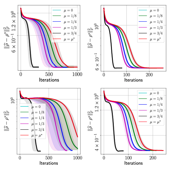
MiFGD performance on real quantum data from IBM QPU. Top-left: GHZminus(6), Top-right: GHZminus(8), Bottom-left: Hadamard(6), Bottom-right: Hadamard(8).

Above figure summarizes the performance of \(\texttt{MiFGD}\). In the legends, \(\mu^\star\) is the momentum parameter proposed by our theory; however, it should be noted that \(\texttt{MiFGD}\) converges with larger momentum values than \(\mu^\star\), in particular featuring a steep dive to convergence for the largest value of \(\mu\) we tested. Moreover, the above figure also highlights the universality of our approach: its performance is oblivious to the quantum state reconstructed, as long as it satisfies purity or it is close to a pure state. Our method does not require any additional structure assumptions in the quantum state.

It should be noted that quantum data are inherently noisy. To highlight the level of noise existing in real quantum data, in the figure below, we also plot the performance of \(\texttt{MiFGD}\) in the same setting using simulated quantum data from IBM’s QASM simulator:

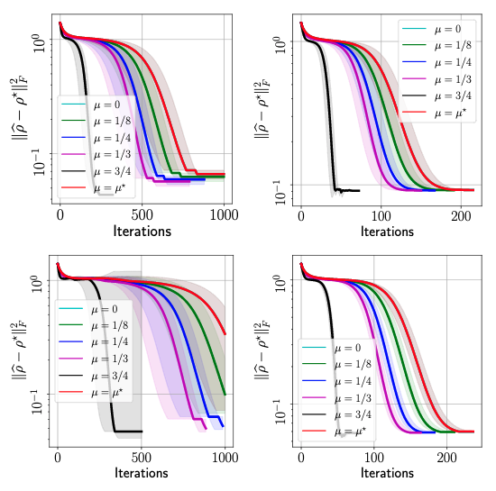
MiFGD performance on synthetic data using IBM’s QASM simulator. Top-left: GHZminus(6), Top-right: GHZminus(8), Bottom-left: Hadamard(6), Bottom-right: Hadamard(8).

We see a similar trend with the result using real quantum data from IBM’s QPU. However, we see that the overall accuracy of the reconstucted and the target states, \(\|\hat{\rho} - \rho^\star\|_F^2\), is generally lower for the real quantum data–they do not reach the accuracy level of \(10^{-1}\), which is acchieved for all cases using QASM simulator. This difference is summarized in the figure below:

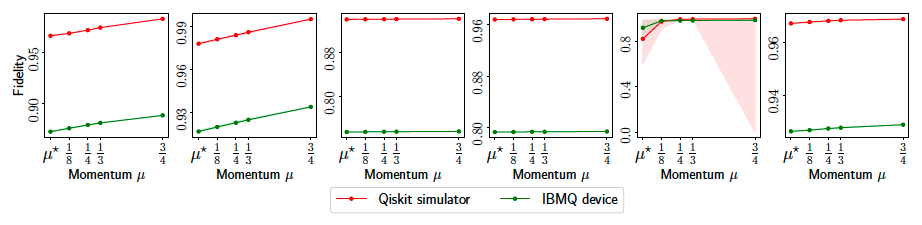
Final fidelity of MiFGD comparison using real quantum data from IBM’s QPU and simulated quantum data using QASM.

Performance comparison with QST methods in $\texttt{Qiskit}$

Now, we compare the performance of \(\texttt{MiFGD}\) with QST methods from \(\texttt{Qiskit}\), again using IBM’s QASM simulator. \(\texttt{Qiskit}\) provides two QST methods: \(i)\) the \(\texttt{CVXPY}\) method which relies on convex optimiztion, and \(ii)\) the \(\texttt{lstsq}\) which ruses least-squares fitting. Both methods solve the following full tomography problem (not compressed sensing QST problem):

\begin{align} \min_{\rho \in \mathbb{C}^{d \times d}} \quad & f(\rho) := \tfrac{1}{2} ||\mathcal{A}(\rho) - y||_2^2 \quad \text{subject to} \quad & \rho \succeq 0, ~\texttt{Tr}(\rho) = 1. \end{align}

We note that \(\texttt{MiFGD}\) is not restricted to “tall” \(U\) scenarios to encode PSD and rank constraints: even without rank constraints, one could still exploit the matrix decomposition \(\rho = UU^\dagger\) to avoid the PSD projection, \(\rho \succeq 0\), where \(U \in \mathbb{C}^{d \times d}\).

We consider the following cases: \(\texttt{GHZ}(n), \texttt{Hadamard}(n),\) and \(\texttt{Random}(n)\) for \(n = 3, \dots, 8\). The results are shown in the figure below:

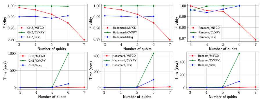
Performance comparison with Qiskit methods. All experiments are performed on a 13” Macbook Pro with 2.3 GHz Quad-Core Intel Core i7 CPU and 32 GB RAM.

Some notable remarks: \(i)\) For small-scale scenarios (\(n=3, 4\)), \(\texttt{CVXPY}\) and \(\texttt{lstsq}\) attain almost perfect fidelity, while being comparable or faster than \(\texttt{MiFGD}\). \(ii)\)The difference in performance becomes apparent from \(n = 6\) and on: while \(\texttt{MiFGD}\) attains \(98\)% fidelity in less than \(5\) seconds, \(\texttt{CVXPY}\) and \(\texttt{lstsq}\) require up to hundreds of seconds to find a good solution. Finally, while \(\texttt{MiFGD}\) gets to high-fidelity solutions in seconds for \(n = 7, 8\), \(\texttt{CVXPY}\) and \(\texttt{lstsq}\) methods require more than 12 hours execution time; however, their execution never ended, since the memory usage exceeded the system’s available memory.

Performance comparison with neural-network QST using \(\texttt{Qucumber}\)

Next, we compare the performance of \(\texttt{MiFGD}\) compare with neural-network based QST methods, proivded by \(\texttt{Qucumber}\). We consider the same quantum states as with \(\texttt{Qiskit}\) experiments, but here we consider the case where only \(50\)% of the measurements are available.

We report the fidelity of the reconstruction as a function of elapsed training time for \(n = 3, 4\) in the figure below for all methods provided by \(\texttt{Qucumber}\): \(\texttt{PRWF}, \texttt{CWF}\), and \(\texttt{DM}\). Note that Time (secs) on \(x\)-axis is plotted with log-scale.

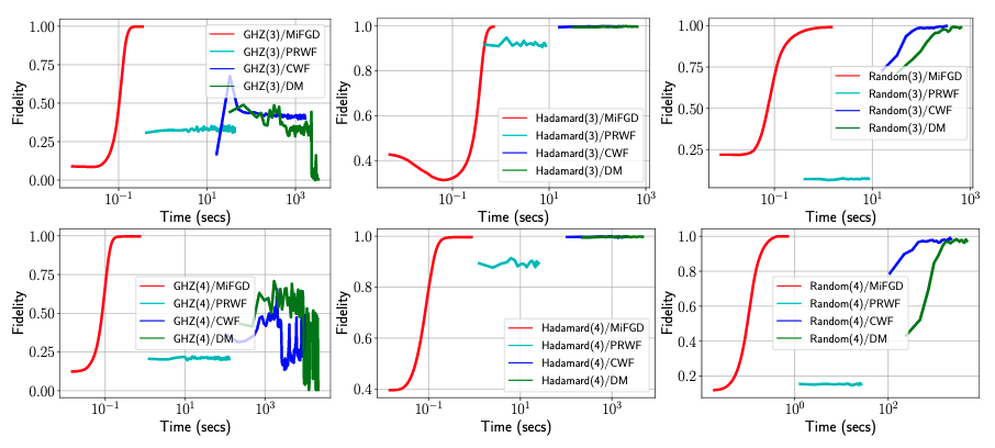
Performance comparison with Qucumber methods. All experiments are performed on a NVidia GeForce GTX 1080 TI with 11GB RAM.

We observe that for all cases, \(\texttt{Qucumber}\) methods are orders of magnitude slower than \(\texttt{MiFGD}\). For the \(\texttt{Hadamard}(n)\) and \(\texttt{Random}(n)\), reaching reasonable fidelities is significantly slower for both \(\texttt{CWF}\) and \(\texttt{DM},\) while \(\texttt{PRWF}\) hardly improves its performance throughout the training. For the \(\texttt{GHZ}\) case, \(\texttt{CWF}\) and \(\texttt{DM}\) also shows non-monotonic behaviors: even after a few thousands of seconds, fidelities have not “stabilized”, while \(\texttt{PRWF}\) stabilizes in very low fidelities. In comparison, \(\texttt{MiFGD}\) is several orders of magnitude faster than both \(\texttt{CWF}\) and \(\texttt{DM}\) and fidelity smoothly increases to comparable or higher values. What is notable is the scalability of \(\texttt{MiFGD}\) compared to neural network approaches for higher values of \(n\).

To see this more clearly, in the table below, we report the final fidelities (within the \(3\) hour time window), and reported times. We see that for many cases, \(\texttt{CWF}\) and \(\texttt{DM}\) methods did not complete a single iterations within \(3\) hours.

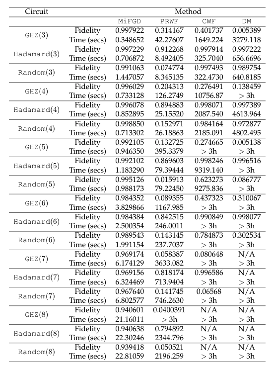
Comparison with Qucumber methods.

The effect of parallelization in \(\texttt{MiFGD}\)

We also study the effect of paralleization in running \(\texttt{MiFGD}\). We parallelize the iteration step across a number of processes, that can be either distributed and network connected, or sharing memory in a multicore environment. Our approach is based on Message Passing Interface (MPI) specification. We assign to each process a subset of the measurement labels consumed by the parallel computation. At each step, a process first computes the local gradient using a subset of measurements. These local gradients are then communicated so that they can be added up to form the full gradient, and the full gradient is shared with each worker.

In our first round of experiments, we investigate the scalability of the parallelization approach. We vary the number \(p\) of parallel processes \((p=1, 2, 4, 8, 16, 32, 48, 64, 80, 96)\), collect timings for reconstructing \(\texttt{GHZ}(4)\), \(\texttt{Random}(6)\) and \(\texttt{GHZminus}(8)\) states, and report speedups \(T_p/T_1\) we gain from \(\texttt{MiFGD}\) in the figure bloew (left panel). We observe that the benefits of parallelization are pronounced for bigger problems (here: \(n=8\) qubits) and maximum scalability results when we use all physical cores ($48$$ in our platform).

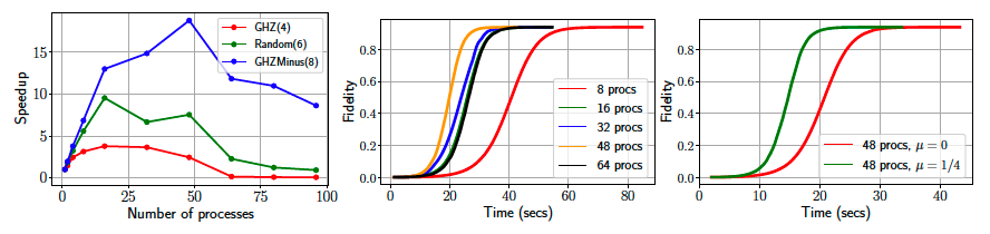
Effect of parallelization of MiFGD. Left: scalability of parallelization of MiFGD for different number of processors. Middle: fidelity versus time consued for different number of processors on Hadamard(10) state. Right: The effect of momentum on Hadamard(10) state with 48 processors.

Further, we move to larger problems (\(n=10\) qubits: reporting on reconstructing \(\texttt{Hadamard}(10)\) state) and focus on the effect parallelization to achieving a given level of fidelity in reconstruction. In the middle panel of the figure above, we illustrate the fidelity as a function of the time spent in the iteration loop of \(\texttt{MiFGD}\) for (\(p=8, 16, 32, 48, 64\)): we observe the smooth path to convergence in all \(p\) counts which again minimizes compute time for \(p=48\). Note that in this case we use \(10\)% of the complete measurements, and the momenutum parameter \(\mu=\frac{1}{4}\).

Finally, in the right panel of the figure above, we fix the number of processes to \(p=48\), in order to minimize compute time and increase the percentage of used measurements to \(20\)% of the complete measurements available for \(\texttt{Hadamard}(10)\). We vary the momentum parameter from \(\mu=0\) (no acceleration) to \(\mu=\frac{1}{4}\), and confirm that we indeed get faster convergence times in the latter case while the fidelity value remains the same (i.e. coinciding upper plateau value in the plots). We can also compare with the previous fidelity versus time plot, where the same \(\mu\) but half the measurements are consumed: more measurements translate to faster convergence times (plateau is reached roughly \(25\)% faster; compare the green line with the yellow line in the previous plot).

Conclusion

We have introduced the \(\texttt{MiFGD}\) algorithm for the factorized form of the low-rank QST problems. We proved that, under certain assumptions on the problem parameters, \(\texttt{MiFGD}\) converges linearly to a neighborhood of the optimal solution, whose size depends on the momentum parameter \(\mu\), while using acceleration motions in a non-convex setting. We demonstrate empirically, using both simulated and real data, that \(\texttt{MiFGD}\) outperforms non-accelerated methods on both the original problem domain and the factorized space, contributing to recent efforts on testing QST algorithms in real quantum data. These results expand on existing work in the literature illustrating the promise of factorized methods for certain low-rank matrix problems. Finally, we provide a publicly available implementation of our approach, compatible to the open-source software \(\texttt{Qiskit}\), where we further exploit parallel computations in \(\texttt{MiFGD}\) by extending its implementation to enable efficient, parallel execution over shared and distributed memory systems.

back

1. Junhyung Lyle Kim, George Kollias, Amir Kalev, Ken X. Wei, Anastasios Kyrillidis. Fast quantum state reconstruction via accelerated non-convex programming. arXiv preprint arXiv:2104.07006, 2021. ↩ ↩² ↩³

2. D. Gross, Y.-K. Liu, S. Flammia, S. Becker, and J. Eisert. Quantum state tomography via compressed sensing. Physical review letters, 105(15):150401, 2010. ↩

3. A. Kalev, R. Kosut, and I. Deutsch. Quantum tomography protocols with positivity are compressed sensing protocols. NPJ Quantum Information, 1:15018, 2015. ↩

4. Giacomo Torlai, Guglielmo Mazzola, Juan Carrasquilla, Matthias Troyer, Roger Melko, and Giuseppe Carleo. Neural-network quantum state tomography. Nat. Phys., 14:447–450, May 2018. ↩

5. Giacomo Torlai and Roger Melko. Machine-learning quantum states in the NISQ era. Annual Review of Condensed Matter Physics, 11, 2019. ↩

6. Matthew JS Beach, Isaac De Vlugt, Anna Golubeva, Patrick Huembeli, Bohdan Kulchytskyy, Xiuzhe Luo, Roger G Melko, Ejaaz Merali, and Giacomo Torlai. Qucumber: wavefunction reconstruction with neural networks. SciPost Physics, 7(1):009, 2019. ↩

7. D. Gonçalve, M. Gomes-Ruggiero, and C. Lavor. A projected gradient method for optimization over density matrices. Optimization Methods and Software, 31(2):328–341, 2016. ↩

8. E. Bolduc, G. Knee, E. Gauger, and J. Leach. Projected gradient descent algorithms for quantum state tomography. npj Quantum Information, 3(1):44, 2017. ↩

9. Jiangwei Shang, Zhengyun Zhang, and Hui Khoon Ng. Superfast maximum-likelihood reconstruction for quantum tomography. Phys. Rev. A, 95:062336, Jun 2017. ↩

10. Zhilin Hu, Kezhi Li, Shuang Cong, and Yaru Tang. Reconstructing pure 14-qubit quantum states in three hours using compressive sensing. IFAC-PapersOnLine, 52(11):188 – 193, 2019. 5th IFAC Conference on Intelligent Control and Automation Sciences ICONS 2019. ↩

11. Zhibo Hou, Han-Sen Zhong, Ye Tian, Daoyi Dong, Bo Qi, Li Li, Yuanlong Wang, Franco Nori, Guo-Yong Xiang, Chuan-Feng Li, et al. Full reconstruction of a 14-qubit state within four hours. New Journal of Physics, 18(8):083036, 2016. ↩

12. A. Kyrillidis, A. Kalev, D. Park, S. Bhojanapalli, C. Caramanis, and S. Sanghavi. Provable quantum state tomography via non-convex methods. npj Quantum Information, 4(36), 2018. ↩ ↩² ↩³

13. Benjamin Recht, Maryam Fazel, and Pablo A Parrilo. Guaranteed minimum-rank solutions of linear matrix equations via nuclear norm minimization. SIAM review, 52(3):471–501, 2010. ↩