The question
Most of the abilities a modern reasoning model has are bought with more parameters. Bigger models, more weights, more roles. The question we asked is the inverse: can one set of weights play more than one role on its own?
The setting is small recurrent Transformers — networks that read a puzzle, then quietly turn it over in their heads for a fixed number of cycles before answering. A recent paper, the Hierarchical Reasoning Model (HRM), showed that this kind of architecture — only a few million parameters, but allowed to recur — can do surprisingly well on hard combinatorial puzzles like Sudoku-Extreme and 30×30 mazes. HRM's recipe is structural: it carries two latent recurrent states, a high-level z_H and a low-level z_L, and assigns each to its own Transformer with its own parameters. The two networks, the paper reports, end up doing visibly different things.
A follow-up paper (the Tiny Recursive Model, TRM) made a striking observation: you don't need two networks. Replace both with a single shared Transformer that's called twice per cycle, and the model still works. So a natural question follows. If the two recurrent states are now driven by identical parameters, do they still develop distinct roles? Or does the shared model treat the two updates as essentially the same operation?
Our paper, with Jucheng Shen and Barbara Su, asks this question carefully and answers it: yes, specialization survives the move to a single shared model — but only when the model has some way to tell which of the two states it is currently updating. The most minimal such signal, and the one we focus on, is whether the encoded input is injected into the update at all.
A minimal architecture
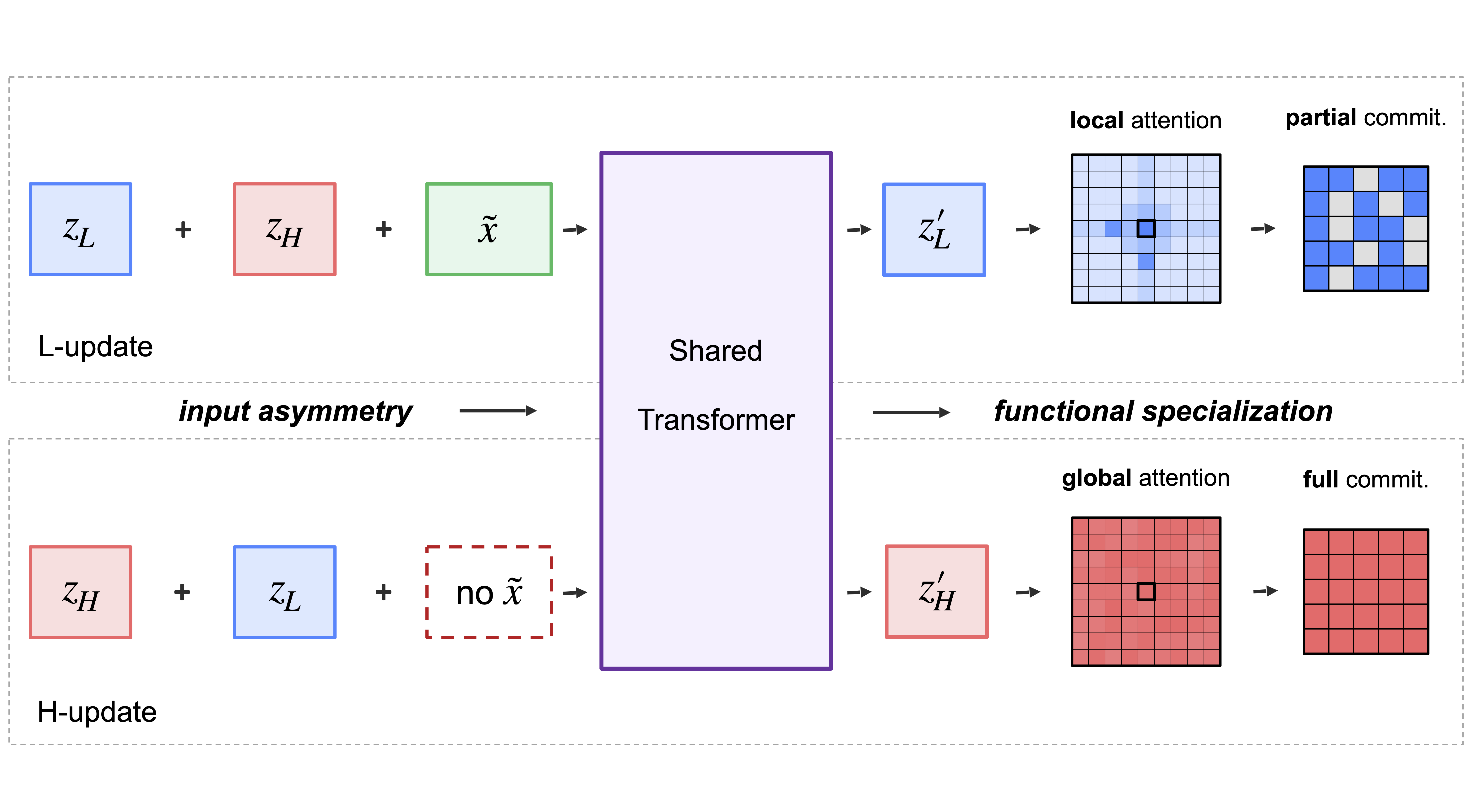
The architecture, which we call AIR (Asymmetric Input Recurrence), keeps the two-state scaffold of HRM but ties the two updates to a single Transformer block. Per cycle it performs six sub-steps in a fixed pattern — L, L, H, L, L, H — and the gradient is taken only through the last L and the last H of each cycle, so backpropagation traverses the shared block exactly twice per training step. The only difference between the two update types is built into the input wiring:
Both updates use the same Transformer \(f(\cdot;\theta)\); the encoded input \(\tilde{\mathbf{x}}\) appears in one and is absent from the other. Nothing else distinguishes them. The output head sits on top of z_H, so the training signal supervises z_H directly while z_L is shaped only by the recurrence. Each Transformer is four layers, eight heads, hidden dimension 512 — deliberately small.
The encoded input \(\tilde{\mathbf{x}}\) is a deterministic, structured function of the puzzle tokens. So the two update types — "with \(\tilde{\mathbf{x}}\)" and "without" — occupy distinguishable regions of the shared block's input space. A sufficiently expressive Transformer can therefore implement two different update maps by conditioning on the presence or absence of \(\tilde{\mathbf{x}}\). That is an existence statement. The rest of the paper asks whether training actually finds such a separation, and what it looks like when it does.
What the two states do
To see what each state is doing, we use the trick that mechanistic-interpretability work has been using for some time: apply the trained output head not just to the final z_H, but to every intermediate state, at every sub-step, and read out what the model would have said if asked to stop right then. The output is a Sudoku grid in one experiment and a maze in the other. We can look.
Sudoku
The decoded picture is consistent across puzzles and across the five random seeds we trained. z_H always renders a complete Sudoku board — every cell filled with a digit, even when several of those digits are still wrong. z_L renders an incomplete board — some cells held back as a special BLANK token while the model is still uncertain about them — and the locations of those held-back cells shift across sub-steps as the puzzle is worked.
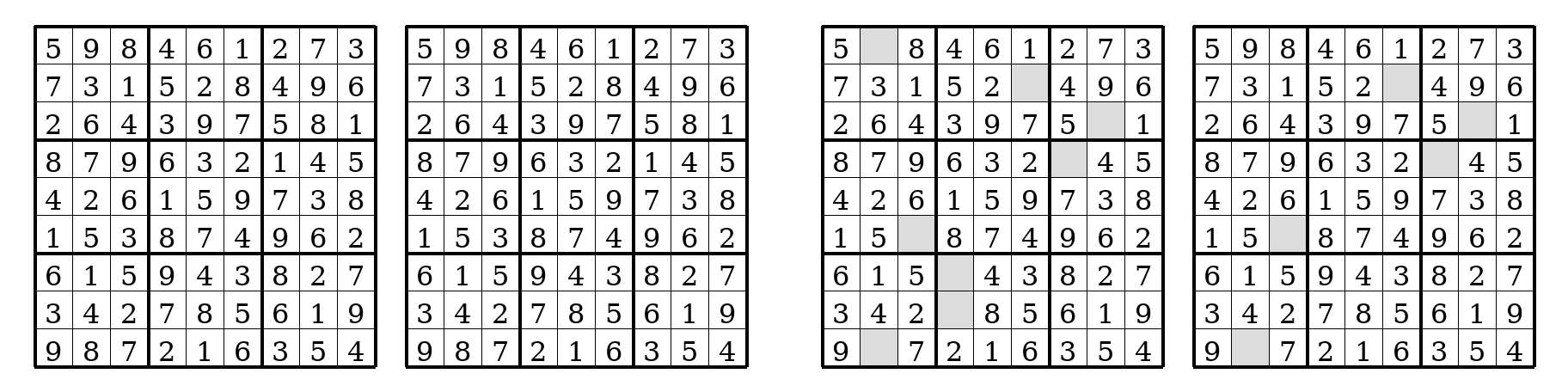
BLANK, with the held-back set changing from one sub-step to the next.
Maze
The same split appears on 30×30 maze navigation, in the vocabulary appropriate to that task. z_H commits to a complete layout of walls, paths, and solution. z_L leaves regions undecided (the PAD token) and rearranges its uncertainty locally as the rollout progresses.
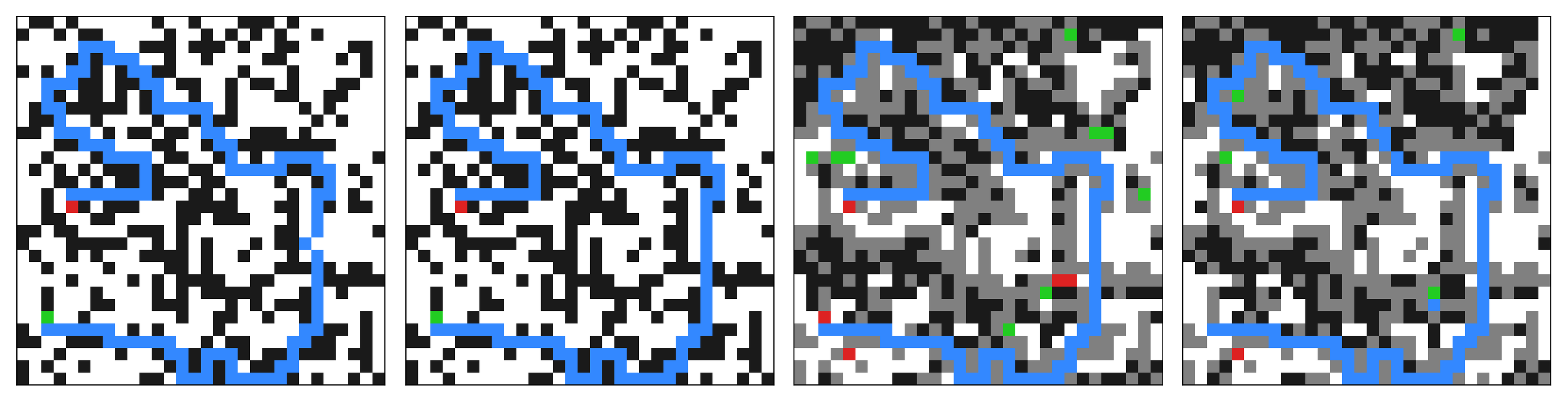
PAD). z_H commits; z_L hesitates and revises.
What if the asymmetry were removed?
The cleanest test of whether the asymmetry is doing the work is to take it away. We trained a symmetric variant — call it Lx_Hx — in which the input \(\tilde{\mathbf{x}}\) is injected into both the L- and the H-update with equal weight. Same number of parameters, same architecture, same training procedure. The only thing different is the input wiring.
The decoded division of labour goes away.
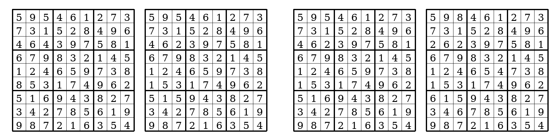
BLANK pattern of Figure 2, and z_H loses its early commitment. The two states look like two copies of the same thing.
The same flattening happens on Maze, in its own vocabulary: the symmetric z_L no longer shows the PAD-bearing intermediate structure of Figure 3; the two states converge to versions of the same picture.
So the picture above is not just a consequence of having two recurrent buffers and a recurrent training schedule. It is a consequence of the one architectural detail that makes the two update types distinguishable to the shared model.
The numbers
What does this asymmetry buy? We measured final test accuracy across a small grid of input-injection configurations, varying \((n_L, n_H)\) — the number of copies of \(\tilde{\mathbf{x}}\) added to each update type. The asymmetry level is \(\Delta = |n_L - n_H|\), so the symmetric controls have \(\Delta = 0\) and the canonical AIR variants have \(\Delta = 1\) or \(\Delta = 2\). All numbers are mean ± standard deviation across five training seeds, evaluated on the full held-out test set (422,786 Sudoku puzzles; 1,000 mazes).
| Variant | (n_L, n_H) | Δ | Sudoku (%) | Maze (%) |
|---|---|---|---|---|
| Asymmetric (Δ > 0) | ||||
| L_Hx | (0, 1) | 1 | 58.7 ± 3.3 | 75.3 ± 3.2 |
| Lx_H (default) | (1, 0) | 1 | 60.0 ± 2.0 | 71.0 ± 6.3 |
| L_H2x | (0, 2) | 2 | 58.6 ± 1.9 | 75.6 ± 1.9 |
| L2x_H | (2, 0) | 2 | 59.1 ± 2.4 | 71.1 ± 6.4 |
| Lx_H2x | (1, 2) | 1 | 59.6 ± 0.9 | 70.9 ± 2.4 |
| L2x_Hx | (2, 1) | 1 | 58.6 ± 2.9 | 74.5 ± 1.6 |
| Group mean | — | — | 59.1 | 73.1 |
| Symmetric (Δ = 0) | ||||
| Lx_Hx | (1, 1) | 0 | 52.1 ± 1.6 | 69.4 ± 2.5 |
| L2x_H2x | (2, 2) | 0 | 50.9 ± 2.9 | 70.3 ± 4.2 |
| Group mean | — | — | 51.5 | 69.9 |
| Two-network baseline (separate parameters) | ||||
| HRM (Wang et al. 2025) | — | — | 55.0 | 74.5 |
The pattern is the same on both tasks: every asymmetric configuration sits above every symmetric one. On Sudoku the gap is roughly eight points (~59% vs ~51.5%); on Maze it is narrower but in the same direction (~73% vs ~70%). And the best AIR variants are also at or above the original two-network HRM baseline — Sudoku +5 points, Maze +1 point — with half the parameter count, since the L- and H-Transformers are now one shared block instead of two.
The Sudoku gap is real and replicates across seeds. The Maze gap is smaller and the within-group spread is wider — some asymmetric configurations (Lx_H, L2x_H, Lx_H2x) are statistically indistinguishable from the symmetric ones. We don't claim asymmetric input is universally better on Maze; we claim the directional effect is consistent, and that the best asymmetric configurations match the two-network baseline at half the parameters.
Can a different signal do the same job?
The follow-up question is whether input injection specifically is the load-bearing part, or whether any signal that tells the shared model "you are doing an L-update right now" would do. We tested this by starting from the symmetric base and adding a small learned level token in three different ways:
| Variant | Mechanism | Sudoku (%) |
|---|---|---|
| L2x_H2x (base, no token) | — | 50.9 ± 2.9 |
| + Addition | element-wise add to every token | 50.0 ± 1.9 |
| + Prepend (strip) | prepend, attend, then strip | 57.5 ± 1.3 |
| + Prepend (no strip) | prepend, persist across cycles | 47.8 ± 1.6 |
| For reference: asymmetric Δ=1 | — | ~59.0 |
The patterns are revealing. Element-wise addition of a level vector to every content token does nothing — the signal is mixed in with the content and the shared model cannot disentangle it. Prepending a level token but letting it persist across cycles is worse than the symmetric base, presumably because the persistent token accumulates content and so the per-sub-step signal is no longer clean. What works is the structurally cleanest of the three: prepend the level token, let it participate in self-attention, then strip it out before the next sub-step. That variant recovers a substantial fraction of the asymmetric-injection benefit and lifts the symmetric base by ~7 points.
Are the two states related?
It is one thing for two states to look different when you decode them. It is another for those states to be doing complementary work — for each one to be holding up some part of the computation that the other depends on. We test this directly. During inference, we freeze one of the two states (hold it constant across sub-steps) and let the other update normally, then measure how the unfrozen state behaves.
The metric is what we call content change: the number of decoded-token positions that change from one sub-step to the next. Lots of content change means the unfrozen state is busily revising; little change means it has gone quiet.
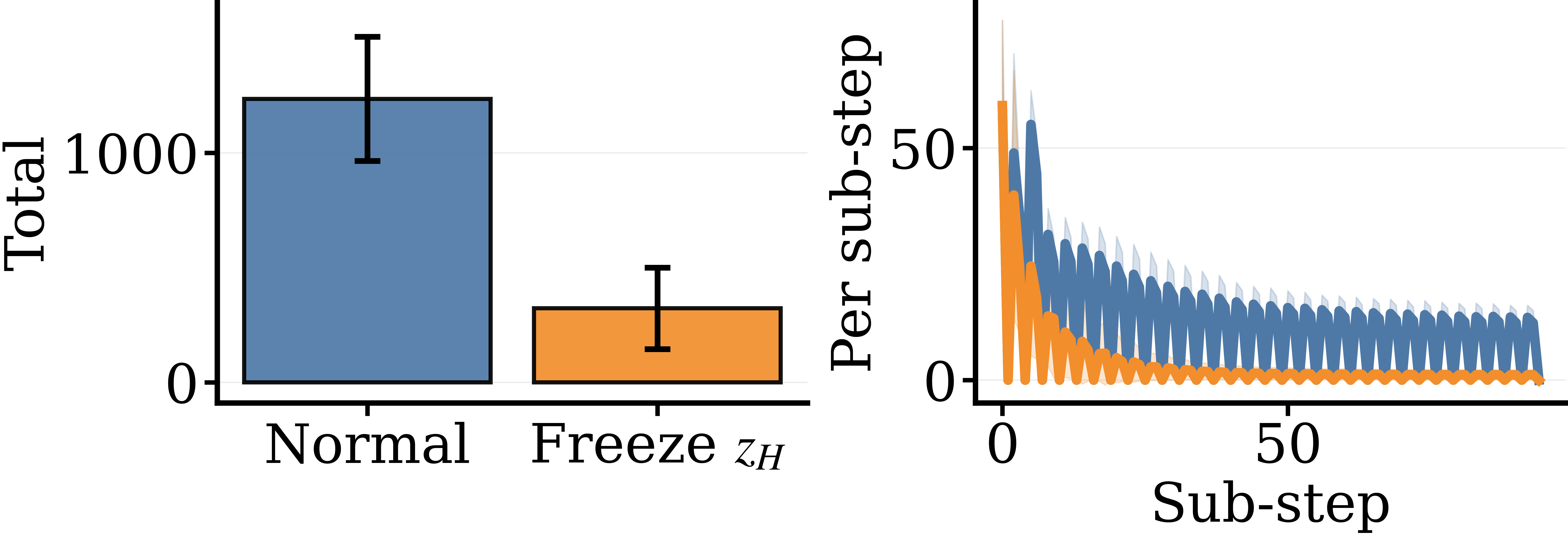
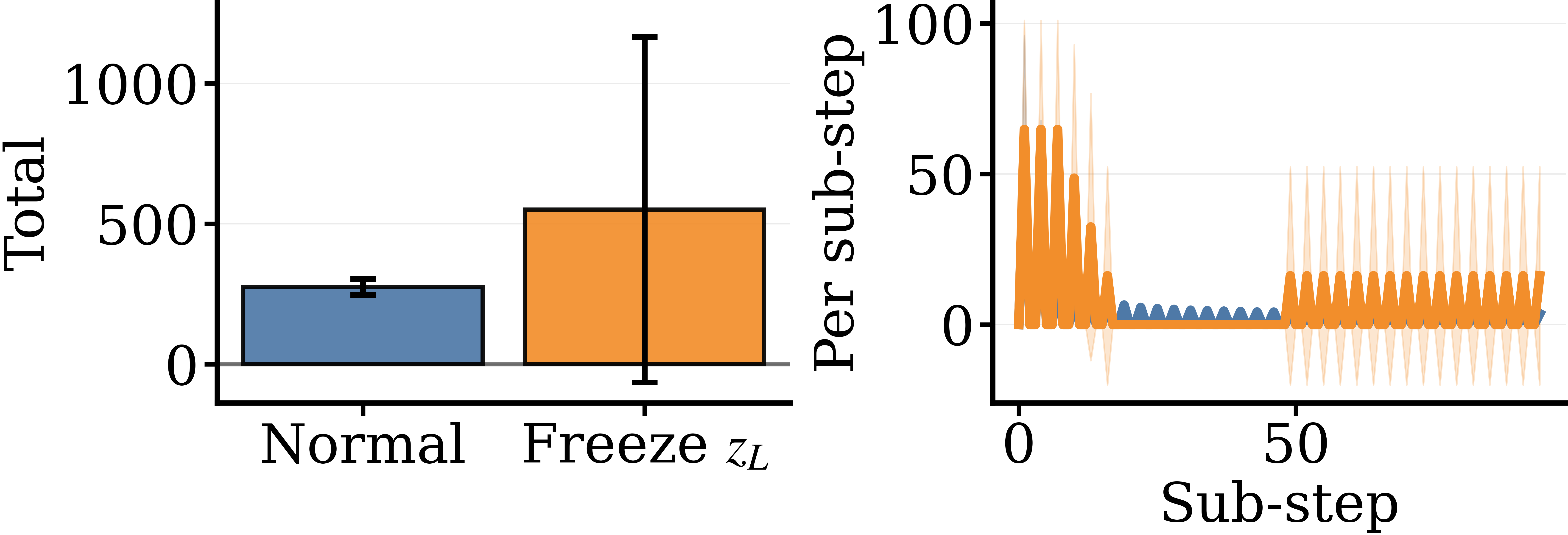
On Sudoku the dynamics tell a coherent story: z_H is in some sense the driver of z_L's revisions — take z_H away and z_L goes quiet — while z_L is in some sense the stabilizer of z_H — take it away and z_H flails. They are not two parallel buffers; they are two ends of a feedback loop.
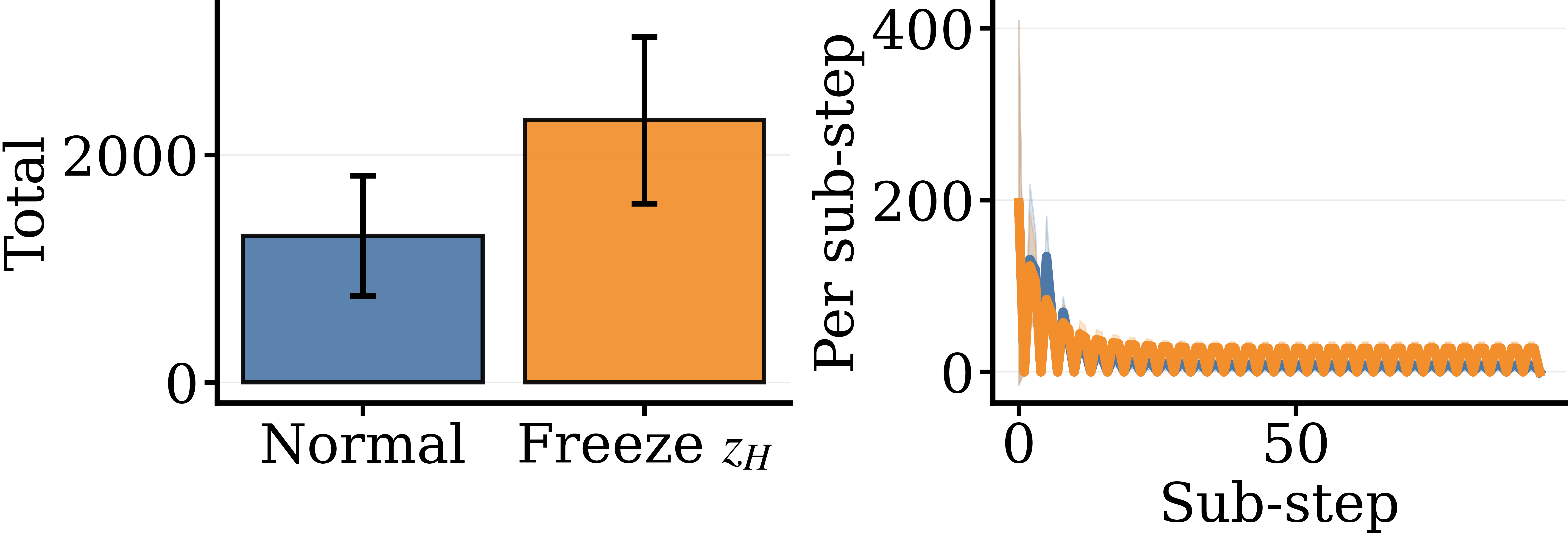
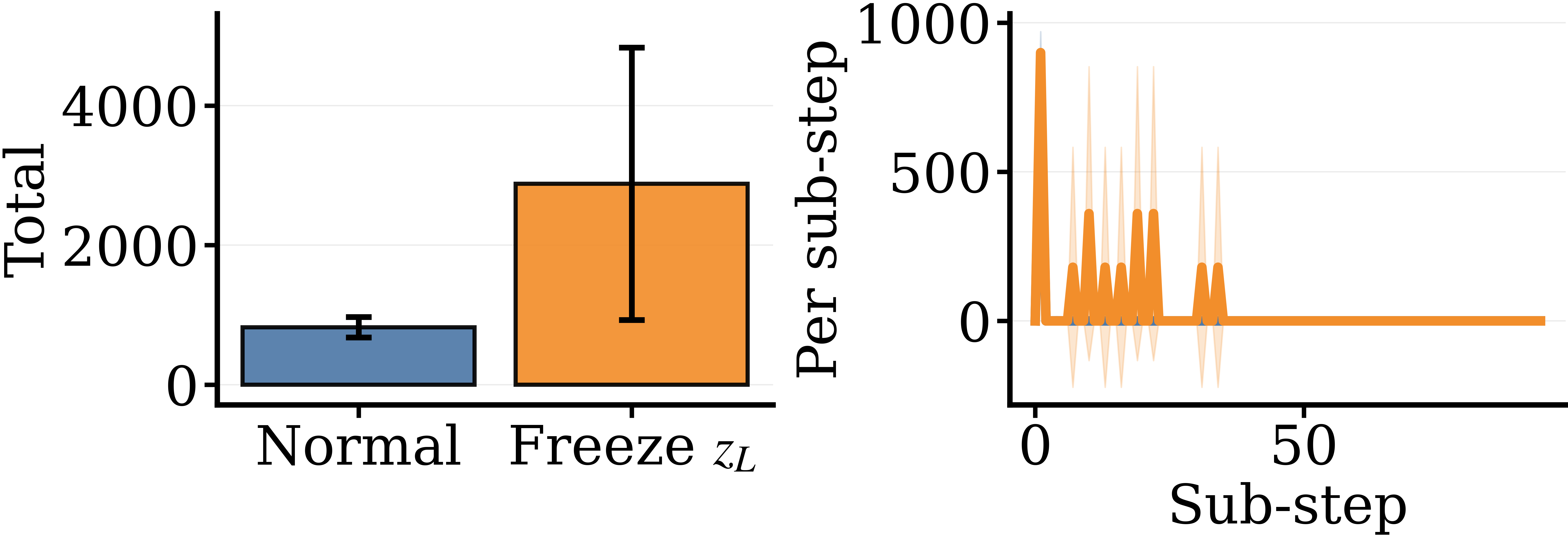
On Maze the picture is symmetric in shape but opposite in sign: freezing either state amplifies the other's revisions. The two tasks differ in the geometry of their state coupling — Sudoku's seems hierarchical, Maze's seems mutual — but in both, the freeze tests demonstrate that the two states are doing complementary work. The decoded role split is not just a visual artefact; it is a property of how the model's dynamics depend on each part.
The symmetric Lx_Hx control, by contrast, does not show this organized freeze response — freezing either state in the symmetric model produces unstructured perturbation rather than a role-consistent pattern. The two pictures are coherent only when the asymmetry is present.
Freezing either state collapses final task accuracy to zero on both Sudoku and Maze. The asymmetric model is not just a proposal network with a decorative scratchpad — every part is load-bearing.
The mechanism: local and global
The decoded behaviour and the freeze responses are downstream of something happening inside the Transformer. To get at that, we looked at the attention. Each sub-step has its own attention pattern; we measured, for every blank query cell, how much attention mass lands inside the cell's local neighbourhood, and compared the L-update with the H-update.
On Sudoku, every blank cell has a natural neighbourhood: the twenty other cells that share its row, its column, or its 3×3 box — the cells whose values constrain it. Before any aggregate statistics, it is worth looking at a single example.
p0121, query r2c6) in the first cycle, viewed at the shallowest layer. The L-update places about 0.81 of its attention mass inside the constraint neighbourhood (the same row, column, and 3×3 box as the query); the H-update places only 0.24. Same puzzle, same query, same head — only the update type differs.
The picture above is not cherry-picked geometry; the same pattern recurs on different puzzles and different queries. Here is a second example, where L's attention happens to concentrate along the query's row inside the neighbourhood, while H's attention drifts off-board:
p0025, cycle 4, query r1c3). The local-versus-global split survives a change of puzzle, cycle, head, and query cell.
To check that this is not an artefact of a particular sub-step or a particular cycle, we tracked one query cell, head, and layer across the full cycle schedule. The L/H separation persists; it is a property of which update type is being performed, not of when.
p0829, query r1c9) tracked across cycles 2 through 15. At every cycle, the L-update (top row) attends more locally and the H-update (bottom row) attends more globally. The role assignment is not a one-cycle artefact.
Now the aggregate picture. We computed three L−H contrasts at every layer of the Transformer, averaging over the eight attention heads and 1,000 test puzzles:
The largest gap appears at the deepest layer, where L places about 47% more attention mass inside the neighbourhood than H does. The same direction holds at every layer of the network. There is a corresponding entropy gap: L's attention distribution is more concentrated than H's. A second signal — call it the violation signal — looks at whether L attends disproportionately to cells whose current decoded value already conflicts with another cell in the same row/column/box. This signal emerges only in the deeper layers and is small but reliable.
Maze tells the locality half of the same story. We constructed three neighbourhoods of increasing size around each blank cell (4-cardinal, 8-surround, and the centred 5×5 window) and measured the per-cell density contrast between L and H. The density is positive across every neighbourhood size and every layer; the smaller the neighbourhood, the larger the L − H gap.
Two readings:
- Local vs global. When the shared Transformer is asked to update z_L, it attends locally; when asked to update z_H, it attends globally. The split is consistent across both tasks and across all layers we measured.
- Task-specific specialization. Sudoku, whose constraints span the board, additionally develops a deeper-layer signal that routes extra attention to violated cells. Maze, whose interactions are inherently local, does not — once the model attends locally, there is no further signal to add.
The picture in attention is the same picture we saw in the decoded states and in the freeze experiments, just expressed in a different observable. One shared model, two update types, two distinguishable computational behaviours.
Why this matters
There is a common assumption in modern architecture design that if you want a network to play multiple roles, you build it with multiple parameter sets — multiple experts, multiple modules, multiple heads, multiple LoRA adapters. Functional modularity is implemented as parameter modularity, by construction.
What this work suggests, in a small and carefully controlled setting, is that the relationship is more relaxed than that. A single set of parameters can play more than one role if it has a clean signal at update time telling it which role it is in. The signal can be thin — in our case, the mere presence or absence of the input vector is enough. What it cannot be is mixed indistinguishably into the content.
That has two implications worth thinking about. The first is design-economic: the same task can be solved by a model with half the parameters of the obvious modular alternative, if the architecture exposes a sufficient state-identity signal. The second is mechanistic: when we ask what a shared model is "really doing," the answer can be "two different things at two different invocations," and that is detectable by the kinds of probes that mechanistic-interpretability work has been using to read inside transformer LLMs.
It is also a small but pointed counterpoint to a tempting narrative about specialization. Specialization does not need to be hard-wired into the weights; it can be a property the shared weights learn, given a clean enough invocation signal. Whether this scales — to deeper models, to natural-language reasoning, to non-grid combinatorial structure — is the next round of questions.
Honest scope
We are explicit about where this evidence comes from. The experiments use two synthetic, fully observable, grid-structured combinatorial tasks (Sudoku-Extreme with 17 givens; Maze on a 30×30 grid). The model is a 4-layer Transformer with two recurrent latent states and \(C_L = C_H = 2\) sub-steps per cycle. Mechanistic evidence is strongest on Sudoku. Attention weights are only a partial view of what a network is computing. None of this generalizes for free.
What we have shown is that, in this controlled setting, a single shared recurrent block develops stable, related, mechanistically-distinguishable functional roles when its update types are made distinguishable. Whether the same pattern persists in deeper architectures, in language modelling, in partial-observability tasks, in continuous domains — those are the natural next questions, and we have not answered them here.
What we suspect — and we are deliberately stating this as a suspicion, not a finding — is that the principle is more general than the proof. Wherever a network is asked to play multiple roles inside a shared computation, providing a clean per-invocation identity signal is likely to be a cheap and effective way to elicit specialization without paying for it in parameters. That is a hypothesis. The evidence in this paper is suggestive, not conclusive.
1. Beyond grids. Does the proposal-and-scratchpad split survive when tokens are not grid cells — for instance in a small Transformer-LM trained on iterated reasoning?
2. More than two roles. Does \(k > 2\) latent states with \(k\) distinct invocation signals layer cleanly, or do the roles collide?
3. Sharp theory. The universal-approximation argument is only an existence statement. Under what conditions on the data and the optimization does training provably recover the split?
4. Other signals. Position, modality, and conditioning vectors are other forms of asymmetry. Which kinds of identity signal work, and which collapse?