Co-writers: Vatsal Shah, John Chen

Deep learning has been hugely successful in areas such as image classification and speech recognition, where a large amount of labeled data is available. However, in practice it is often prohibitively expensive to create a large, high-quality labeled dataset, due to lack of time and resources, among other factors.^{1 2}

Some common issues that plague the process of labelling include:

• Labelling is time consuming: Creating a labeled dataset often involves months of intense preparations before, during and after the data collection. ImageNet dataset—which consists of 3.2 million labeled images in 5247 categories—took nearly two and half years to complete with the aid of Amazon’s Mechanical Turk.
• The process of data labelling is expensive: Labelling is quite expensive as it involves access to millions of data samples, storing them, crowdsourcing or any other mechanism to collect labels and aggregating these results to get the best quality dataset. A typical dataset would also involve images that are easy and hard to label. For example, it is not reasonable to assume that an average annotater is able to recognize dogs of different breeds as dogs, but lemurs might be misclassified. For such tasks, we often need experts in different areas such as linguistics, zoologists, etc., which further adds to the operation cost.
• Label Aggregation: Aggregating labels from crowdsourced data is a challenging process as is evidenced by an increasing number of papers in this area.³ Aggregating labels is often necessary to avoid attacks from malicious users or bots, who are planning to make an easy buck with minimal effort.

As we know, there are numerous challenges that we encounter in the procurement of high quality labeled datasets. Here, we would like to explore if it is possible to utilize the unlabeled samples, which provides some information about the distribution, with the help of running a toy example. One of the most common issues for supervised learning when there is a lack of data points is the selection bias of the classifier. As we show, it is possible to reduce or eliminate this bias using unlabeled samples.

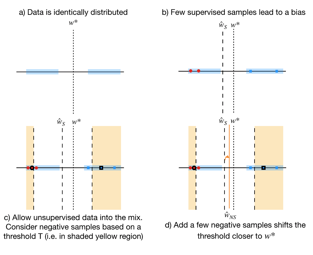
We will consider a simple example in 1D (Figure above), where we assume binary classification with cross-entropy loss for simplicity. Let $w^\star$ denote the separating hyperplane and assume that the data lies uniformly on either side of $w^\star$, indicated by the shaded blue region (top left plot of the figure). Without loss of generality, let the points on the left and right of the hyperplane have the labels $1$ and $0$, respectively. Our aim is to recover $w^\star$.

It is possible for the labeled examples to have a selection bias⁴ (for example certain images of cats are easier to label than others); assume that this property leads the algorithm to converge to $\hat{w}$; see top-right plot of the figure. However, assume that we do have access to a large number of unlabeled examples. How can we utilize it to improve our prediction?

Consider one of the highlighted samples $(x_u)$ (red dot with black boundary in left-bottom plot). Let us assume its underlying true label is $1$. The key difference in both approaches is that we make a gradient update by labeling any point in the shaded yellow region as the predicted label while in negative sampling we make a gradient update by labeling the same point as not $0$. Both these algorithms only perform updates only if we are certain about the label.

Now, let us compare the gradients of a sample using the above algorithms:

\[\text{Approach 1}: \nabla \mathcal{L}\left(\{x_u\}\right) = -(1-\mu_{u}) x_u \\ \text{Approach 2}: \nabla \mathcal{L}\left(\{x_u\} \right) = \mu_{u} x_u\]

From the equations above, it is clear that both approaches push the gradients in opposite directions. The gradient updates of supervised samples align with the gradient updates of the unsupervised samples labeled using Approach 1. However, that is not the case for Approach 2. Since the unsupervised data samples come from a uniform distribution, it is more likely that we will pick more “negative” samples from the class on the right (intersection of yellow and blue shaded regions). These negative samples have a bias to the right side of the plane ultimately bringing back the separating hyper-plane closer to $w^\star$ (bottom-right plot in the figure).

What is Semi-supervised learning?

We have been talking about supervised and unsupervised samples. How can we span the space between the two approachs? The aim of semi-supervised learning (SSL) is to utilize the unlabeled data in conjunction with labeled data to improve the quality of predictions. Chapelle et. al.⁵ provides a detailed survey on semi-supervised learning methods which can be divided into following main topics:

1. Inductive SSL,
2. Transductive SSL

In this blog post, we restrict our attention to a subset of inductive SSL algorithms which add a loss to the supervised loss function. These algorithms tend to be more practical in terms of hyperparameter tuning⁶. There are a number of SSL algorithms not discussed in this blog, including “transductive” models⁷, graph-based methods^{8 9}, and generative modeling^{10 11}. For a comprehensive overview of SSL methods, refer to⁸, or⁵.

Consistency Regularization: Consistency regularization applies data augmentation to semi-supervised learning with the following intuition: Small perturbations for each sample should not significantly change the output of the network. This is usually achieved by minimizing some distance measure between the output of the network, with and without perturbations in the input. This is the general intuition for the current dominant approach in SSL.

Pi Model: The most straightforward distance measure is the mean squared error used by the $\Pi$ model^{12 13}. The $\Pi$ model adds the distance term $d(f_{\theta}(x),f_{\theta}(\hat{x}))$, where $\hat{x}$ is the result of a stochastic perturbation to $x$, to the supervised classification loss as a regularizer, with some weight.

Mean Teacher: Mean teacher¹⁴ observes the potentially unstable target prediction over the course of training with the $\Pi$ model approach, and proposes a prediction function, parameterized by an exponential moving average of model parameter values. Mean teacher adds $d(f_{\theta}(x),f_{\theta ‘}(x))$, where $\theta ‘$ is an exponential moving average of $\theta$, to the supervised classification loss with some weight. The performance of Mean teacher can be boosted with substantial hyperparameter tuning.⁶

Virtual Adversarial Training: Virtual Adversarial Training¹⁵ (VAT) approximates perturbations to be applied over the input to most significantly affect the output class distribution, inspired by adversarial examples.^{16 17} VAT computes an approximation of the perturbation as:

\[r \sim \mathcal{N}\left(0, \tfrac{\xi}{\sqrt{\mathrm{dim}(x)}} I\right)\\ g = \nabla_r d\left(f_{\theta}(x), f_{\theta}(x + r)\right)\\ r_{\text{adv}} = \epsilon \cdot g/\|g\|_2\]

where $x$ is an input data sample, $\text{dim}(\cdot)$ is its dimension, $d$ is a non-negative function that measures the divergence between two distributions, $\xi$ and $\epsilon$ are scalar hyperparameters. Consistency regularization is then used to minimize the distance between the output of the network, with and without the perturbations in the input. It is worth noting adversarial robustness affects the performance of neural networks¹⁸, but it not necessarily relevant to VAT.

Entropy minimization: The goal of entropy minimization¹⁹ is to discourage the decision boundary from passing near samples where the network produces low-confidence predictions. One way to achieve this is by adding a simple loss term to minimize the entropy for unlabeled data $x$ with total $K$ classes: $-\sum_{k=1}^{K} \mu_{xk} \log \mu_{xk}.$ Entropy minimization on its own has not demonstrated competitive performance in SSL, however it can be combined with VAT for stronger results^{15 20}.

Pseudo-Labeling: Pseudo-Labeling²¹ is a simple and easy to tune method which is widely used in practice. For a particular sample, it requires only the probability value of each class, the output of the network, and labels the sample with a class if the probability value crosses a certain threshold. The sample is then treated as a labeled sample with the standard supervised loss function. Pseudo-Labeling is closely related to entropy minimization, but only enforces low-entropy predictions for predictions which are already low-entropy. The popularity of Pseudo-Labeling is likely due to its simplicity and limited extra cost for hyperparameter search.

Mixup based SSL: Mixup ²² combines pairs of samples and their one-hot labels $(x_1, y_1), (x_2, y_2)$ as in: $x’ = \lambda x_1 + (1 - \lambda) x_2, y’ = \lambda y_1 + (1 - \lambda) y_2$, where $\lambda \sim \texttt{Beta}(\alpha, \alpha)$, to produce a new sample $(x’, y’)$ with $\alpha$ being a hyperparameter. Mixup is a form of regularization which encourages the neural network to behave linearly between training examples, justified by Occam’s Razor. In SSL, the labels $y_1, y_2$ are typically the predicted labels by a neural network with some processing steps.

Applying Mixup to SSL led to Interpolation Consistency Training (ICT)²³ and MixMatch⁶, which significantly improved upon previous results with SSL on the standard benchmarks of CIFAR10 and SVHN. ICT trains the model $f_{\theta}$ to output predictions similar to a mean-teacher $f_{\theta ‘}$, where $\theta ‘$ is an exponential moving average of $\theta$. Namely, on unlabeled data, ICT encourages $f_{\theta} (\texttt{Mixup}(x_i, x_j)) \approx \texttt{Mixup}(f_{\theta ‘}(x_i), f_{\theta ‘}(x_j))$.

MixMatch applies a number of processing steps for labeled and unlabeled data on each iteration and mixes both labeled and unlabeled data together. The final loss is given by

\[\mathcal{L} = \mathcal{L}_{\text{supervised}} + \lambda_3 \mathcal{L}_{\text{unsupervised}},\]

where

\[\mathcal{X}', \mathcal{U}' = \texttt{MixMatch}(\mathcal{X}, \mathcal{U}, E, A, \alpha), \\ \mathcal{L}_{\text{supervised}} = \frac{1}{|\mathcal{X}'|} \sum_{i_1 \in \mathcal{X}'} \sum_{k=1}^{K} y_{i_1 k} \log \mu_{i_1 k}, \\ \mathcal{L}_{\text{unsupervised}} = \frac{1}{K|\mathcal{U}'|} \sum_{i_2 \in \mathcal{U}'} \sum_{k=1}^{K} ( y_{i_2 k} - \mu_{i_2 k} ) ^2,\]

where $\mathcal{X}$ is the labeled data ${x_{i_1}, y_{i_1}}_{i_1 = 1}^n,$ $\mathcal{U}$ is the unlabeled data ${x_{i_2}^{u}}_{i_2 = 1}^{n_u} $, $\mathcal{X}’$ and $\mathcal{U}’$ are the output samples labeled by MixMatch, and $E$, $A$, $\alpha$, $\lambda_3$ are hyperparameters.

Given a batch of labeled and unlabeled samples, MixMatch applies $A$ data augmentations on each unlabeled sample $x_{i_2}$, averages the predictions across the $A$ augmentations,

\[p = \frac{1}{A} \sum_{a=1}^{A} f_{\theta}(\texttt{Augment}(x_{i_2}^{u}))\]

and applies temperature sharpening,

\[\texttt{Sharpen}(p, E)_k := \frac{p_k^{1/E}}{\sum_{k=1}^{K} p_k^{1/E}},\]

to the average prediction. $A$ is typically 2 in practice, and $E$ is 0.5. The unlabeled data is labeled with this sharpened average prediction.

Let the collection of labeled unlabeled data be $\mathcal{\widehat{U}}$. Standard data augmentation is applied to the originally labeled data and let this be denoted $\mathcal{\widehat{X}}$. Let $\mathcal{W}$ denote the shuffled collection of $\mathcal{\widehat{U}}$ and $\mathcal{\widehat{X}}$. MixMatch alters Mixup by adding a max operation:

\[\lambda \sim \texttt{Beta}(\alpha, \alpha), \lambda ' = \max(\lambda, 1 - \lambda);\]

it then produces $\mathcal{X}’ = \texttt{Mixup}(\mathcal{\widehat{X}}_{i_1} , W_{i_1})$ and $\mathcal{U}’ = \texttt{Mixup}(\mathcal{\widehat{U}}_{i_2} , W_{i_2 + \mathcal{\widehat{X}} })$.

There are further reincarnations of these two methods^{24 25 26}. The latest line of work from the MixMatch group is FixMatch, which pseudo-labels strong augmentations from the pseudo-labels of weak augmentations. This significantly simplifies the pipeline of methods used in MixMatch, while simultaneously boosting performance.

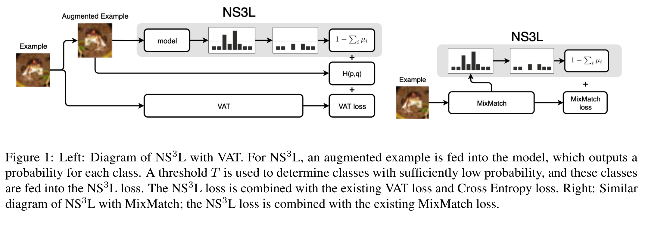
Negative Sampling: Negative Sampling in Semi-Supervised Learning (NS$^3$L)²⁷ is a complementary method to existing state-of-the-art methods in SSL. Instead of encouraging inputs of the same class to cluster together in the latent space, as in consistency regularization, NS$^3$L pushes away inputs from different classes. The particular implementation of NS$^3$L is given by the observation that the Cross Entropy loss can be decomposed as follows. The objective function for cross entropy loss over the labeled examples is:

\[\mathcal{L}\left(\{x_i, y_i\}_{i = 1}^n \right) = - \tfrac{1}{n} \sum_{i = 1}^n \sum_{k = 1}^K y_{ik} \log \mu_{ik},\]

where there are $n$ labeled samples, $K$ classes, $y_{ik} = \mathbb{1}_{k = y_i}$ is the identity operator that equals 1 when $k = y_i$, and $\mu_{ik}$ is the output of the classifier for sample $i$ for class $k$.

For the sake of simplicity, we will perform the following relabeling: for all $i \in [n_u]$, $x_{i+n}=x_i^u$ and $y_{i+n}=y_i^u$. In the hypothetical scenario where the labels for the unlabeled data are known and for $w$ the parameters of the model, the likelihood would be:

\[\mathbb{P}\left[ \{y_i\}_{i = 1}^{n + n_u}~|~\{x_i\}_{i = 1}^{n + n_u}, w \right] = \prod_{i = 1}^{n + n_u} \mathbb{P}\left[ y_i~|~x_i, w \right] = \prod_{i = 1}^{n + n_u} \prod_{k = 1}^K \mu_{ik}^{y_{ik}} = \left( \prod_{i_1 = 1}^{n} \prod_{k = 1}^K \mu_{i_1k}^{y_{i_1k}}\right) \cdot \left (\prod_{i_2 = 1}^{n_u} \prod_{k = 1}^K \mu_{i_2k}^{y_{i_2k}^u} \right)\]

Observe that, $\prod_{k = 1}^K \mu_{i_2k}^{y_{i_2k}^u} = 1 - \sum_{j: y_{i_2 j} \neq 1} \mu_{i_2 j}$, which follows from the definition of the quantities $\mu_{:}$ that represent a probability distribution and, consequently, sum up to one.

Taking negative logarithms allows us to split the loss function into two components: $i)$ the supervised part and $ii)$ the unsupervised part. The log-likelihood loss function can now be written as follows:

\[\mathcal{L}\left( \{ x_i, y_i\}_{i = 1}^{n + n_u} \right) = - \underbrace{\tfrac{1}{n} \sum_{i_1 = 1}^n \sum_{k = 1}^K y_{ik} \log \mu_{ik}}_{:= \text{supervised part}} - \underbrace{\tfrac{1}{n_u} \sum_{i_2 = 1}^{n_u} \log \left(1 - \sum_{j \neq \text{True label}} \mu_{i_2j} \right)}_{:= \text{unsupervised part}}\]

While the true labels need to be known for the unsupervised part to be accurate, we draw ideas from negative sampling/contrastive estimation²⁸²⁹. I.e., for each unlabeled example in the unsupervised part, we randomly assign $P$ labels from the set of labels. These $P$ labels indicate classes that the sample does not belong to: as the number of labels in the task increase, the probability of including the correct label in the set of $P$ labels is small. The way labels are selected could be uniformly at random or by using Nearest Neighbor search, or even based on the output probabilities of the network, where with high probability the correct label is not picked.

In practice, more often than not we train models based on stochastic gradient descent, and we implement a mini-batch variant of this approach with different batch sizes $B_1$ and $B_2$ for labeled and unlabeled data, respectively. Our $\text{NS}^3\text{L}$ loss then looks as:

\[\hat{\mathcal{L}}_{B_1, B_2}\left( \{x_i, y_i\}_{i = 1}^{n + n_u} \right) = -\tfrac{1}{|B_1|} \sum_{i_1 \in B_1} \sum_{k = 1}^K y_{ik} \log \mu_{ik} - \underbrace{\tfrac{1}{|B_2|} \sum_{i_2 \in B_2} \log \left(1 - \sum_{j = 1}^{P_{i_2}} \mu_{i_2 j} \right)}_{:= \text{$\text{NS}^3\text{L}$ loss}}.\]

Thus, the loss is useful if those classes which the input is not can be accurately predicted.

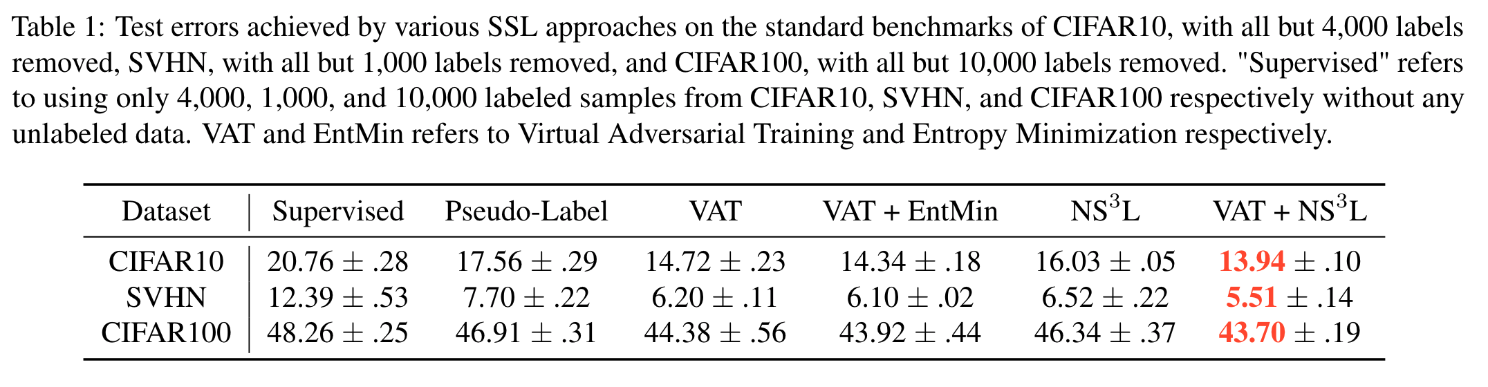
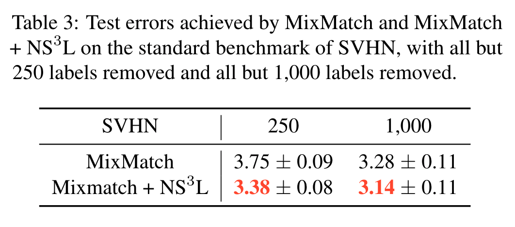
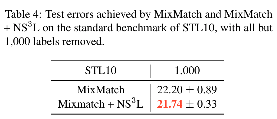
Some results on these state of the art methods We follow the practice in ³⁰ and use the same hyperparameters for plain $\text{NS}^3\text{L}$ and $\text{NS}^3\text{L}$ in $\text{NS}^3\text{L}$ + VAT for both CIFAR10 and SVHN. After selecting hyperparameters on CIFAR10 and SVHN, we run almost the exact same hyperparameters with little further tuning on CIFAR100, where the threshold $T$ is divided by 10 since there are 10x classes in CIFAR100.

The results are shown below for non-Mixup-based SSL settings:

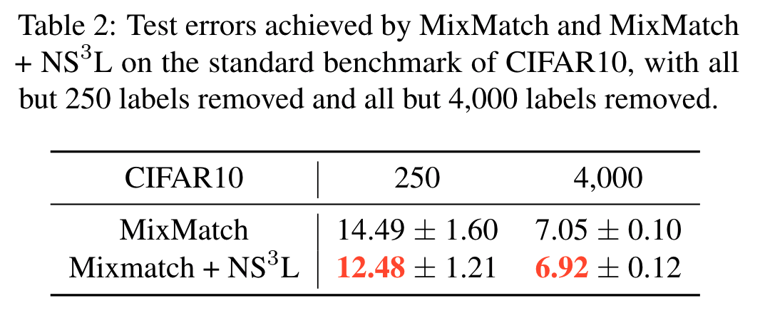
Below you can find some results for Mixup-based SSL settings:

A systems’ schema for negative sampling in SSL

Conclusion

In this blog post, we introduced the most popular works in the dominant approach of consistency regularization for SSL today. We covered the Pi model, Mean Teacher, VAT, Mixup based models, and NS$^3$L approaches. Hopefully this blog was helpful for getting you up to speed with the state-of-the-art for SSL and provide some intuition to why they work.