Introduction to quantum computing: From classical to quantum (part I).

Sources: “Quantum computing for computer scientists”, N. Yanofsky and M. Mannucci, Cambridge Press, 2008.

This is part of a (probably) long list of posts regarding quantum computing. In this post, we will take the leap from classical to quantum notions.

Disclaimer: while the material below might seem too simple for some scientists, I suggest not skimming over this post - personally, I always enjoy reading something that I believe I own, as επαναληψη μητηρ πασης μαθησεως (repetition is the mother of any knowledge)

A rough description of a quantum system

We will start a bit abruptly by defining what a quantum system is. I will try not to use math yet in this first description of a quantum system and its state.

Let’s roughly say that a quantum system is a system (think of it as a computational unit), characterized by:

• the number of qubits $n$ (for the moment, think of computer bits, but they are quite different),
• its initial state, which is represented as a complex vector in $\mathbb{C}^{2^n}$.
• a collection of registers, each one of which is associated with a qubit (thus, we must have at least $n$ in our architecture), and each one directly interacts with all or a subset of the rest registers (qubits), based on a couple mapping of the quantum computer architecture.

When we say quantum computing, we (very very very) roughly mean that:

• We have access to a quantum computer¹.
• We start from a specific state, that we choose. Essentially, the initial state is the input to the quantum computer.
• We carefully select a series of operations, that often correspond to multiplying a quantum state with a unitary matrix. The result of each multiplication corresponds to an intermediate quantum state.
• The combination of the initial state and the set of operations we choose correspond roughly to a definition of an algorithm, through quantum tools and nomenclature.
• The final state is the output of the system, that we measure and that we hope is the answer to the problem we want to solve.

Once again, this is a very rough description, based on my understanding so far. This might change as we progress more into the details.

¹ This reminds me of an excellent saying/quote I read in a CS book: “Recipe for the best dragon soup: first, find a dragon…“.

The analogy with the dynamics of a graph

Here, following the book of Yanofsky and Mannucci, we make the analogy between a quantum system and the evolution of a Markov chain in action over a graph.

Probabilistic system

Let us borrow the following example from Wikipedia. Consider the following state diagram.

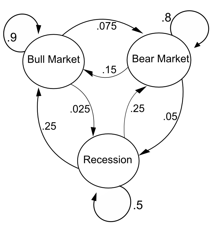
The states represent whether a hypothetical stock market is exhibiting a bull market, bear market, or stagnant market trend during a given week. According to the figure, a bull week is followed by another bull week 90% of the time, a bear week 7.5% of the time, and a stagnant week the other 2.5% of the time.

One can represent the “system” through the matrix of transitions.

\[\mathbf{P} = \begin{bmatrix} 0.9 & 0.075 & 0.025 \\ 0.15 & 0.8 & 0.05 \\ 0.25 & 0.25 & 0.5 \end{bmatrix}.\]

W.l.o.g., we lable the state space as 1 = bull, 2 = bear, 3 = stagnant. Let us also assume that the state we are at is the vector:

\[\mathbf{x}_0 = \begin{bmatrix} 0 \\ 1 \\ 0 \end{bmatrix},\]

i.e., we are at the bear state.

To measure the dynamics of the system, given the current state, we would like to see what happends in the next time click (= week). This corresponds to applying the operation $P$ on the current state.

\[\mathbf{x}_1 = \mathbf{P} \mathbf{x}_0 = \begin{bmatrix} 0.9 & 0.15 & 0.25 \\ 0.075 & 0.8 & 0.25 \\ 0.025 & 0.05 & 0.5 \end{bmatrix} \cdot \begin{bmatrix} 0 \\ 1 \\ 0 \end{bmatrix} = \begin{bmatrix} 0.15 \\ 0.8 \\ 0.05 \end{bmatrix}.\]

I.e., with probability 0.8 we will have another bear week, etc.

If we would like to see what happens to the week after that, we re-apply the above rule.

\[\mathbf{x}_2 = \mathbf{P} x_1 = \mathbf{P} (\mathbf{P} \mathbf{x}_0) = \mathbf{P}^2 \mathbf{x}_0 \\ = \begin{bmatrix} 0.8275 & 0.2675 & 0.3875 \\ 0.13375 & 0.66375 & 0.34375 \\ 0.03875 & 0.06875 & 0.26875 \\ \end{bmatrix} \cdot \begin{bmatrix} 0 \\ 1 \\ 0 \end{bmatrix} = \begin{bmatrix} 0.2675 \\ 0.66375 \\ 0.06875 \end{bmatrix}.\]

In both cases, the application of the transition matrix is represented as a matrix-vector multiplication; using $\mathbf{P}$ as a basic operation, it is possible to calculate, for example, the long-term fraction of weeks during which the market is stagnant, or the average number of weeks it will take to go from a stagnant to a bull market.

Let us now make the analogy with the rough description of a quantum system we provided above: the initial state of a quantum system is something like $\mathbf{x}_0$ above, the operations/computations are the transition matrices $\mathbf{P}$ (we will see that in quantum systems we have a collection of operations we can apply), and the final outcome is the outcome after applying a series of matrix-vector products to the original state.

Further, the use of a stochastic graph (i.e., going from one state to another is not a deterministic fact; it depends on the probability of selecting paths from the current state to the next) is perfect for the analogy of the inherent indeterminacy in our knowledge of a physical quantum state.

Overall:

• Vector states express a type of indeterminacy about the exact state of the system (where we actually are).
• Operation matrices are interconnected with the actual dynamics of the system (how we change from one state to another).
• Operations can be simulated as sequential matrix multiplications.

Complex probabilistic system

Now, let us make a further step towads quantum systems. Quantum states are represented as complex vectors. While in the graph analogy, states are real vectors, with entries representing probabilities that sum up to one, in quantum systems, states are complex vectors, where the sum of modulus values squared sum up to one.

Let’s see how this differs in an abstract sense. Again, we are far from describing a real quantum machine, so whatever we discuss below sound… vacuous. Assume $x_i = 1/3$ represent a probability; i.e., the probability of the event $x_i$ is $1/3$. Let also $x_j$ be another event with probability $1/5$. Observe that these numbers are in $[0, 1]$ and can be, for instance, entries of a state in a graph. An obvious but critical observation is that the probability of either events $x_i, x_j$ is the addition of the individual probabilities $x_i + x_j = 8/15$. The following two obvious rules naturally apply:

\[x_i + x_j \geq x_i,\]

and

\[x_i + x_j \geq x_j.\]

You might wonder: “this is one of the most obvious thing I’ve ever read”. And I agree with you.

Let us now move to a case where probabilities are represented as the modulus of a complex number. Consider again a complex number $c_i = \tfrac{1}{4} + i \tfrac{1}{2}$ with corresponding “probability” $x_i = |c_i|^2 = 0.3125$. Also, let $c_j = -\tfrac{1}{3} - i \tfrac{1}{4}$ with “probability” $x_j = |c_j|^2 = 0.17361$. However, if we add the two events $c_k = c_i + c_j$, the corresponding “probability” is: $x_k = |c_k|^2 = 0.069444$. I.e. complex numbers can cancel each other and result into lower “probability”. This has a well-defined meaning in quantum mechanics: interference. But we will discuss this further as we proceed; for the moment, have in mind that a graph with complex numbers as “probabilities”/weights behaves differently than a graph with real numbers as probabilities/weights.

Let’s consider an example; see the following transition graph.

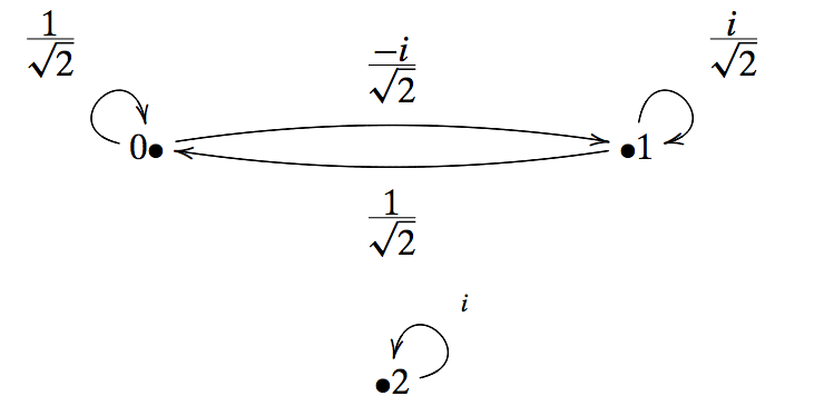
Consider a graph with 3 nodes and a transition matrix as follows:

\[\mathbf{U} = \begin{bmatrix} \tfrac{1}{\sqrt{2}} & \frac{1}{\sqrt{2}} & 0 \\ \tfrac{-i}{\sqrt{2}} & \frac{i}{\sqrt{2}} & 0 \\ 0 & 0 & i \end{bmatrix}\]

Observe that the transition matrix, instead of being a doubly stochastic one, it is unitary. In general, unitary matrices are related to doubly stochastic matrices as follows: the modulus squared of all the entries of a unitary matrix form a doubly stochastic matrix. I.e,

\[|\mathbf{U}|^2 = \begin{bmatrix} \tfrac{1}{2} & \frac{1}{2} & 0 \\ \tfrac{1}{2} & \frac{1}{2} & 0 \\ 0 & 0 & 1 \end{bmatrix}\]

Given a state vector $\mathbf{x} = \left[\tfrac{1}{\sqrt{3}}, \tfrac{2i}{\sqrt{15}}, \sqrt{\frac{2}{5}}\right]^\top$, we have:

\[\mathbf{U} \mathbf{x} = \mathbf{y} := \begin{bmatrix} \frac{5 + 2i}{\sqrt{30}} \\ \frac{-2 -i \sqrt{5}}{\sqrt{30}} \\ i\sqrt{\frac{2}{5}} \end{bmatrix}\]

Observe that the sum of the modulus squares of $y$ is 1.

Some properties of the unitary transformation matrices:

• If $\mathbf{U}$ represents the evolution of the state from time $t$ to time $t+1$, its adjoint $\mathbf{U}^\dagger$ represents the evolation of the state in the past from time $t$ to time $t-1$.

The take-home message is that dealing problems with complex numbers probably requires a different approach from us. Since quantum systems and computing is inherently complex-based, we need to be aware of these differences.

In the second part of this post, we will describe the double-slit experiment that, $(i)$ summarizes the above information in a toy example, and $(ii)$ describes the connection between classical and quantum states and transitions.