Introduction to quantum computing: The Deutsch algorithm.

Sources:

“Quantum computing for computer scientists”, N. Yanofsky and M. Mannucci, Cambridge Press, 2008.

This is part of a (probably) long list of posts regarding quantum computing.

So far we defined quantum states and systems; we saw some complex logic and how quantum states entail complex information; we discussed about the notion of entanglement and the representation of states via the Bloch diagram. Now, it is time to start introducing simple and intuitive algorithms that show quantum information might be superior over classic bit information.

Disclaimer I: while the material below might seem too simple for some scientists, I suggest not skimming over this post - personally, I always enjoy reading something that I believe I own, as επαναληψη μητηρ πασης μαθησεως (repetition is the mother of any knowledge)

The problem setting

Let us consider the following problem: There is a univariate function $f$, defined over the binary alphabet ${0, 1}$, with output range in the same alphabet ${0, 1}$. I.e., $f : {0, 1} \longrightarrow {0, 1}$.

With a bit of inspection, and making no assumptions about $f$, there are four possible configurations for the function $f$:

• Both inputs $0, 1$ are mapped to the output $0$: $f(0) = f(1) = 0$.
• Both inputs $0, 1$ are mapped to the output $1$: $f(0) = f(1) = 1$.
• Inputs pass through $f$ unchanged: $f(0) = 0$ and $f(1) = 1$.
• Inputs are exchanged after passing through $f$: $f(0) = 1$ and $f(1) = 0$.

We will call the first two cases as $f$ being “constant” (i.e., whatever input we insert, the function behaves the same way), and the last two cases as $f$ being balanced.

The question is the following: Given a function $f : {0, 1} \longrightarrow {0, 1}$ and without knowing anything more than that, determine whether $f$ is a constant or a balanced function with the minimum number of function evaluations.

What a classic algorithm would do?

In the classical sense, an algorithm that solves this problem would implement an if-then-else statement:

if f(0) = 0:
	if f(1) = 0:
		print("Constant")
	else: 
		print("Balanced")
else:
	if f(1) = 0:
		print("Balanced")
	else: 
		print("Constant")

As you can see, we require two function evaluations to figure out the answer. In the next sections, we will see how we exploit superposition of states in quantum machines to solve the problem more efficiently.

Quantum representation: first attempt

For simplicity, we will make the assumption that $f$ maps inputs as: $f(0) = 1$ and $f(1) = 0$. But we will pretend we do not know that this is $f$; similar logic can be derived for other cases of $f$. The above behavior –assuming we represent bits as vectors

can be represented as:

We can easily check that mulptilying on the right with any of $|0\rangle$ or $|1\rangle$ we get $|1\rangle$ and $|0\rangle$ respectively.

We define the following quantum circuit:

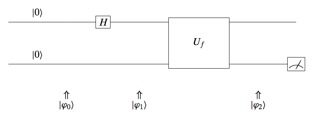
Let us describe what we see in the picture. Initially, the system is as state:

Remember that when we concatenate two 1-qubit states, we get the following 2-qubit representation:

Then, the top input is first transformed through a Hadamard operator to get:

Then, we apply the $U_f$ transformation. With a slight abuse of notation and knowing that $U_f$ applies only on the top input to define the output at the bottom output $| y \oplus f(x) \rangle$, (in a way, the top input is used to evaluate the function $f$ and the bottom input controls the bottom output), $|\mathbf{\varphi}_2\rangle$ becomes:

If we measure the top output, we get 50-50 chance to find in either states; similarly for the bottom qubit. Thus, the above give us no information regarding the nature of $f$. But, we will soon see how we can use this combined with the next subsection.

Quantum representation: second attempt

Let us now consider a different setting for our problem.

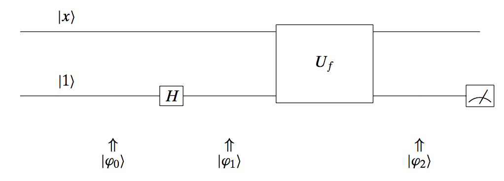
Here, we leave the top input as it is, but we transform the bottom input – which we set to $|1\rangle$ – with a Hadamard matrix.

Let’s go over this circuit and check its state at its time slot. At the beginning, we have:

Using the Hadamard transform, at the next time “click” we obtain the state:

After applying the function operation (remember, it applies only to the second input) we get:

This results into the following “if-then-else” state for $|\mathbf{\varphi}_2 \rangle$:

A more succinct way of writing it is:

Once again, let’s see whether measuring the top or the bottom qubit help us at all: it turns out that again, we cannot figure out the nature of the function $f$ with this circuit configuration, by just using the output.

Quantum representation: third attempt and the Deutsch algorithm

Now, we end up with the final setting, that will lead us to the Deutsch algorithm. See the following diagram:

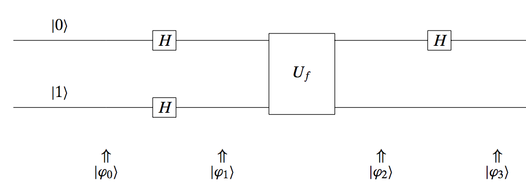
Let us go through the circuit. We start with the state:

Both inputs go through a Hadamard gate; this results into:

In the next step, we go through the function $f$; remember that this function uses the top input to define the output. So far, the top input has the form:

By using the abstract description of the output of $f$ in the previous attempt, a different way to write that output is:

Then, using this information in our new circuit, we obtain altogether:

Let’s see what happens when we take cases of $f$: in our case, $f(0) = 1$ and $f(1) = 0$. Thus:

Repeating the above procedure for all cases of $f$ (constant or balanced) and using the same circuit architecture, we get the following behavior for $| \mathbf{\varphi}_2 \rangle$:

Now, as a final step, we apply again the Hadamard gate to transform the top qubit as follows:

Now, something weird just happened: by just measuring the first qubit we can distinguish whether the function is balanced or constant. And we do this by just one function evaluation (along with other transformations but the bottleneck/constraint here was the number of times we apply $f(\cdot)$.)

While this is a toy example and someone would say “who cares?”, this is actually one of the evidences that someone can achieve exponential acceleration, compared to classical computers.

Extension to multivariate functions: The Deutsch-Jozsa algorithm

Let us make things a bit more interesting by extending the above toy example to multivariate functions. Consider functions $f : {0, 1}^n \rightarrow {0, 1}$. Observe that in this case, the cardinality of input values is exponential: there are $2^n$ different input configurations.

Similar to the previous chapter, we are interested in distinguishing whether $f$ is constant or balanced. Here, constant $f$ is defined as the case where all the inputs are mapped to either 0 or 1. Balanced $f$ is referred to the case where half the input go to 0, and the other half goes to 1. And, for the rest of this discussion, assume that we are assured that the function is either balanced or constant.

Let’s consider first the difficulty of solving this problem with a classical computer. Of course, in the fortunate case where we test two inputs and they give different outputs, we can safely declare that the function is balanced. But, what happens when we continuously get the same output? In that case, we need to check more than half inputs to be sure that the function is constant: i.e., $\frac{2^{n}}{2} + 1 = 2^{n-1} + 1$; still exponential number of inputs and function evaluations.

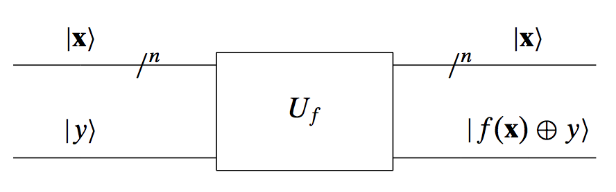
We will describe here succinctly, without much detail, how we would solve this problem using quantum systems with a single function evaluation! Similarly to the univariate input case, now we consider a circuit where the top input is a $n$-dimensional binary string, say $\mathbf{x}$, and the top input is a single qubit $y$. The function evaluation is again denoted with its matrix $U_f$ and the outputs are exactly as depicted in the following (as we will see, failling) circuit attempt:

Similarly to the univariate case, we will need Hadamard matrices to put inputs into superposition. One can define multidimensional Hadamard matrices, by combining single qubit Hadamard matrices. The pattern of defining a $n$-dimensional Hadamard matrix, say $H^{\otimes n}$, is through its kronecker product with itself. E.g., given

we can compute:

Now, we have all the required tools to solve the problem. In order not to make this post huge (however, I found it really interesting to go over the math), we will just present the final circuit that leads to distinguishing a constant vs. balanced binary valued function in just one function evaluation! Here it is:

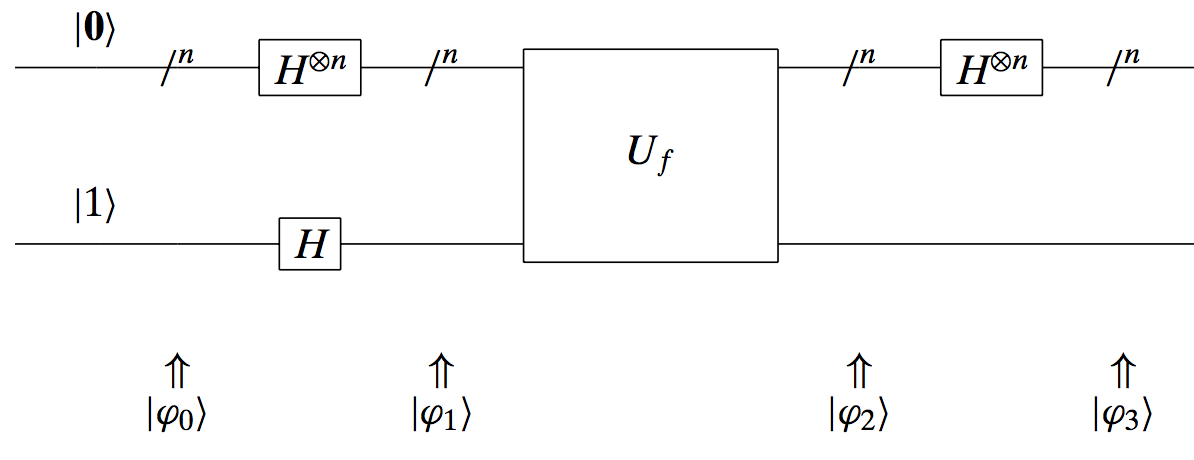
This circuit defines the Deutsch-Jozsa algorithm: i.e., the generalization of the Deutsch algorithm for the multivariate binary case. The final outcome is that if we measure the top qubit in the circuit above, we will only get $|\mathbf{0} \rangle$ if the function is constant! In any other case, it is balanced. And we did so with only one function evaluation: exponential speed-up…