Telling a story about IHT using Python (Chapter I)
The purpose of this notebook is 2-fold: $(i)$ Since this is the first attempt to “migrate” from Matlab-type-of-mathematical-programming language to Python language, this very first notebook serves as a guide for future posts. $(ii)$ This is a loooong post that presents Iterative Hard Thresholding (IHT) algorithm and its variants, a method that solves Compressive Sensing problems in the non-convex setting.
The story is divided in several parts in order to help readability.
Some background on Compressed Sensing (CS) [1-3]. Consider the following underdetermined linear inverse problem: a high-dimensional signal $ \mathbf{x}^\star \in \mathbb{R}^p$ is observed through a low-dimensional observation vector $\mathbf{y} \in \mathbb{R}^n ~(n < p)$ via: \(\mathbf{y} = \boldsymbol{\Phi} \mathbf{x}^\star + \mathbf{w}.\) In this setting, $\boldsymbol{\Phi} \in \mathbb{R}^{n \times p}$ represents the sensing matrix and $\mathbf{w} \in \mathbb{R}^n$ is an additive noise term. Given $\mathbf{y}$ and $\boldsymbol{\Phi}$, unconstrained least-squares method is the classic approach to the solution of linear systems by minimizing the data error function $f(\mathbf{x}) \triangleq ||\mathbf{y} - \boldsymbol{\Phi} \mathbf{x}||_2 ^2$. Nevertheless, the reconstruction of $\mathbf{x}^\star$ from $\mathbf{y}$ is an ill-posed problem since $n < p$ and there is no hope in finding the true vector without ambiguity; additional prior information is needed. In CS, we assume that $\mathbf{x}^\star$ is a sparse vector, i.e., $||\mathbf{x}||_0 \leq k$ where $k \ll p$ and $||\cdot||_0$ is the $\ell_0$-“norm” that counts the non-zero entries of a vector. It turns out that, under proper assumptions on the sensing matrix $\boldsymbol{\Phi}$ and the sparsity level $k$, one can still recover $\mathbf{x}$!
Why sparsity?
Let us consider the following practical case: image processing. In particular, we will see in practice how sparsity appears in digital image representation.
Our first example includes Mario’s favorite food!
import numpy as np
import scipy as sp
import matplotlib.pyplot as plt
import random
from scipy import stats
from scipy.optimize import fmin

from PIL import Image

# Open image using Image package
x_mush_orig = Image.open("mushroom.png").convert("L")
# Transform to a np array
x_mush_star = np.fromstring(x_mush_orig.tobytes(), np.uint8)
# Set the shape of np array
x_mush_star.shape = (x_mush_orig.size[1], x_mush_orig.size[0])
# Show the image
plt.imshow(x_mush_star, interpolation = "nearest", cmap = plt.cm.gray)
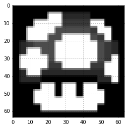
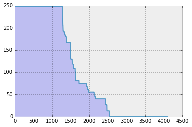
Obviously, this is a simple image case: the “mushroom” image is sparse by itself (do you see the black pixels? Yes, they are zeros). To see this more clearly, let’s sort the true coeffients in decreasing order.
from bokeh.plotting import figure, show, output_file
from bokeh.palettes import brewer

# Get the absolute value of a flatten array (vectorize)
x_mush_abs = abs(x_mush_star.flatten())
# Sort the absolute values (ascending order)
x_mush_abs.sort()
# Descending order
x_mush_abs_sort = np.array(x_mush_abs[::-1])

plt.style.use('bmh')
fig, ax = plt.subplots()
# Generate an array with elements 1:len(...)
xs = np.arange(len(x_mush_abs_sort))
# Fill plot - alpha is transparency (might take some time to plot)
ax.fill_between(xs, 0, x_mush_abs_sort, alpha = 0.2)
# Plot - alpha is transparency (might take some time to plot)
ax.plot(xs, x_mush_abs_sort, alpha = 0.8)
plt.show()
For this 64 x 64 image, the total number of pixels sums up to 4096. As you can observe, by default almost half of the pixels are zero, which constitutes “mushroom” image sparse (but still the sparsity level is quite high: more than half the ambient dimension).
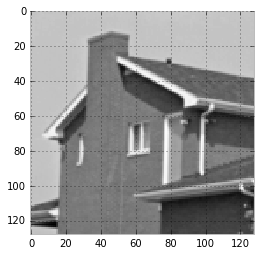
Since this seems to be a “cooked”-up example, let us consider a more realistic scenario: a brick house. (Does anyone know where is this house located?)
x_house_orig = Image.open("house128.png").convert("L")
x_house_star = np.fromstring(x_house_orig.tobytes(), np.uint8)
x_house_star.shape = (x_house_orig.size[1], x_house_orig.size[0])
plt.imshow(x_house_star, interpolation = "nearest", cmap = plt.cm.gray)
…and here is the bar plot of the coefficients.
x_house_abs = abs(x_house_star.flatten())
x_house_abs.sort()
x_house_abs_sort = np.array(x_house_abs[::-1])

plt.style.use('bmh')
fig, ax = plt.subplots()
xs = np.arange(len(x_house_abs_sort))
ax.fill_between(xs, 0, x_house_abs_sort, alpha = 0.2)
plt.plot(xs, x_house_abs_sort, alpha=0.8)
plt.show()
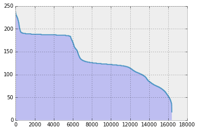
In the plot above, all the coefficients are non-zero! Is there anything we can do in this case?
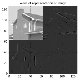
It turns out that, under proper orthonormal transformations,
natural images become sparse. In this simple tutorial, we use wavelets [4-5] (“better” orthonormal transformations could
lead to sparsest solutions, but for ease of exposition and implementation, I use here pywt Python package.)
The wavelet settings for our simple example are:
- Daubechies wavelet family:
db1 - Filters length: 2
- Other properties: Orthogonal, biorthogonal, asymmetric.
import pywt

x_house_orig = Image.open("house.png").convert("L")
x_house_star = np.fromstring(x_house_orig.tobytes(), np.uint8)
x_house_star.shape = (x_house_orig.size[1], x_house_orig.size[0])

# Defines a wavelet object - 'db1' defines a Daubechies wavelet
wavelet = pywt.Wavelet('db1')

# Multilevel decomposition of the input matrix
coeffs = pywt.wavedec2(x_house_star, wavelet, level=2)
cA2, (cH2, cV2, cD2), (cH1, cV1, cD1) = coeffs

# Concatenate the level-2 submatrices into a big one and plot
x_house_star_wav = np.bmat([[cA2, cH2], [cV2, cD2]])
plt.imshow(np.flipud(x_house_star_wav), origin='image', interpolation="nearest", cmap=plt.cm.gray)
plt.title("Wavelet representation of image", fontsize=10)
plt.tight_layout()
After wavelet transformation, let’s plot the wavelet coefficients.
# Flatten and show the histogram
x_house_abs_wav = abs(x_house_star_wav.flatten())
x_house_abs_wav.sort()
x_house_abs_wav.flatten()
x_house_abs_wav_sort = np.array(x_house_abs_wav[::-1])

plt.style.use('bmh')
fig, ax = plt.subplots()
xs = np.arange(len(x_house_abs_wav_sort.flatten()))

ax.fill_between(xs, 0, np.flipud(x_house_abs_wav_sort.flatten()), alpha = 0.2)
plt.plot(xs, np.flipud(x_house_abs_wav_sort.transpose()), alpha = 0.8)
plt.show()
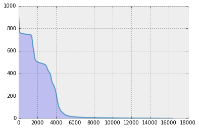
It is obvious that much less number of coefficients are non-zero! (…and this holds generally for natural images.)
from mpl_toolkits.mplot3d import Axes3D
import matplotlib.cm as cm

fig = plt.figure()
ax = fig.add_subplot(111, projection = '3d')
for c, z, zi in zip(['r', 'g', 'b', 'y'], ['house128.png', 'peppers128.png', 'woman128.png', 'lena128.png'], [4, 3, 2, 1]):
    y = Image.open(z).convert("L")
    y_star = np.fromstring(y.tobytes(), np.uint8)
    y_star.shape = (y.size[1], y.size[0])

    # Multilevel decomposition of the input matrix
    y_coeffs = pywt.wavedec2(y_star, wavelet, level=2)
    y_cA2, (y_cH2, y_cV2, y_cD2), (y_cH1, y_cV1, y_cD1) = y_coeffs

    # Concatenate the level-2 submatrices into a big one and plot
    y_star_wav = np.bmat([[y_cA2, y_cH2], [y_cV2, y_cD2]])

    y_abs_wav = abs(y_star_wav.flatten())
    y_abs_wav.sort()
    y_abs_wav.flatten()
    y_abs_wav_sort = np.array(y_abs_wav[::-1])

    xs = np.arange(len(y_abs_wav_sort.flatten()))
    cs = c
    ys = [zi] * len(xs)
    ys = np.array(ys)

    ax.plot(xs, ys = ys.flatten(), zs = np.flipud(y_abs_wav_sort.flatten()), zdir = 'z', color = cs, alpha = 0.5)

ax.set_xlabel('X axis')
ax.set_ylabel('Y axis')
ax.set_zlabel('Z axis')
plt.show
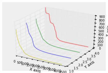
In the above picture, the y values (1.0 to 4.0) correspond to four different image cases (for chanity check, observe that the red curve is the same curve for the house.png case, presented above).
One can observe that most of the coeffs are close to zero and only few of them (compared to the ambient dimension) are significantly large. This has led to the observation that keeping only the most important coefficients (even truncating the non-zero entries further) leads to a significant compression of the image. At the same time, only these coefficients can lead to a pretty good reconstruction of the original image.
Reconstruction of sparse signal from compressive measurements
The discussion above clearly shows that sparsity is present in signal processing (at least in image processing!). And now what? How can one take advantage of this observation? This is where CS theory and algorithms jumps in. As we already stated, CS suggests a type-of compression: given that the signal of interest is sparse, one does not need to observe every entry of $\mathbf{x}$ directly but rather only a compressed version of it, through linear maps. For a more complete discussion on this matter, we defer the blogpost reader to any compressed sensing paper [1-3].
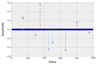
Here, we focus on the task of recovering a sparse signal from such compressive measurements. For the sake of simplicity, we will consider a noiseless case (i.e., $\mathbf{w} = 0$). And also for the sake of simplicity, we will synthetically generate a sparse signal for ease of exposition.
import random
from numpy import linalg as LA

p = 1000  # Ambient dimension
n = 300   # Number of samples
k = 10   # Sparsity level

# Generate a p-dimensional zero vector
x_star = np.zeros(p)
# Randomly sample k indices in the range [1:p]
x_star_ind = random.sample(range(p),  k)
# Set x_star_ind with k random elements from Gaussian distribution
x_star[x_star_ind] = np.random.randn(k)
# Normalize
x_star = (1 / LA.norm(x_star, 2)) * x_star

# Plot
xs = range(p)
markerline, stemlines, baseline = plt.stem(xs, x_star, '-.')
plt.setp(markerline, 'alpha', 0.3, 'ms', 6)
plt.setp(markerline, 'markerfacecolor', 'b')
plt.setp(baseline, 'color', 'r', 'linewidth', 1, 'alpha', 0.3)
plt.xlabel('Index')
plt.ylabel('Amplitude')
plt.show()
For sensing matrix, we assume $\boldsymbol{\Phi}$ satisfies the Restricted Isometry Property:
Definition (Restricted Isometry Property - RIP) [1-3]. An $n \times p$ matrix $\boldsymbol{\Phi}$ satisfies the restricted isometry property for sparsity level $k \geq 1$ if there exists constant $\delta \in (0,1)$ such that the inequalities \((1 - \delta) \|\|\mathbf{x}\|\|\_2 ^2 \leq \|\|\boldsymbol{\Phi} \mathbf{x}\|\|\_2 ^2 \leq (1 + \delta) \|\|\mathbf{x}\|\|\_2 ^2\) hold for all $\mathbf{x} \in \mathbb{R}^p$ with $||\mathbf{x}||_0 \leq k$. The smallest number $\delta \equiv \delta(\boldsymbol{\Phi}, k)$ is called the restricted isometry constant of $\boldsymbol{\Phi}$.
For ease of illustration, we will assume $\boldsymbol{\Phi}$ is drawn entrywise i.i.d. from a Gaussian distribution; see [6] for a proof that subgaussian class of matrices satisfy RIP with high probability.
import math

# Generate sensing matrix
Phi = (1 / math.sqrt(n)) * np.random.randn(n, p)

# Observation model
y = Phi @ x_star
Iterative hard thresholding (IHT) method [7-8]. A natural way to reconstruct $\mathbf{x}^\star$ from $\mathbf{y}$ and $\boldsymbol{\Phi}$ is by solving the criterion: \(\min_{\mathbf{x}} ~~f(\mathbf{x}) := \frac{1}{2}\|\|\mathbf{y} - \boldsymbol{\Phi} \mathbf{x}\|\|\_2 ^2 \quad \text{s.t.} \quad \|\|\mathbf{x}\|\|\_0 \leq k\) Observe that this optimization problem can be solved in a projected gradient descent manner; this is what iterative hard thresholding (IHT) method [7-8] does:
The IHT method
1: Choose initial guess $\mathbf{x}_0$
2: for i = 0, 1, 2, … do
3: Compuete $\nabla f(\mathbf{x}_i) = -\boldsymbol{\Phi}^\top \cdot (\mathbf{y} - \boldsymbol{\Phi} \mathbf{x}_i)$
4: $\mathbf{x}_{i+1} = \mathcal{H}_k\left(\mathbf{x}_i - \nabla f(\mathbf{x}_i)\right)$
5: end for
Here, $\mathcal{H}_k(\cdot)$ denotes the hard thresholding operator: \(\mathcal{H}\_k(\mathbf{w}) \in \arg\min\_{\mathbf{x}:\|\|\mathbf{x}\|\|\_0 \leq k} \frac{1}{2} \|\|\mathbf{x} - \mathbf{w}\|\|\_2 ^2.\) To compute $\mathcal{H}_k(\cdot)$, one needs to find the $k$ largest (in magnitude) elements of the input vector and set the rest to zero. Let’s use this algorithm and see how it performs in practice.
from numpy import linalg as la

# Hard thresholding function
def hardThreshold(x, k):
    p = x.shape[0]
    t = np.sort(np.abs(x))[::-1]
    threshold = t[k-1]
    j = (np.abs(x) < threshold)
    x[j] = 0
    return x

# Returns the value of the objecive function
def f(y, A, x):
    return 0.5 * math.pow(la.norm(y - Phi @ x, 2), 2)

def IHT(y, A, k, iters, epsilon, verbose, x_star):
    # Length of original signal
    p = A.shape[1]
    # Length of measurement vector
    n = A.shape[0]
    # Initial estimate
    x_new = np.zeros(p)
    # Transpose of A
    At = np.transpose(A)

    # Initialize
    x_new = np.zeros(p)           # The algorithm starts at x = 0

    PhiT = np.transpose(Phi)

    x_list, f_list = [1], [f(y, Phi, x_new)]

    for i in range(iters):
        x_old = x_new

        # Compute gradient
        grad = -PhiT @ (y - Phi @ x_new)

        # Perform gradient step
        x_temp = x_old - grad

        # Perform hard thresholding step
        x_new = hardThreshold(x_temp, k)

        if (LA.norm(x_new - x_old, 2) / la.norm(x_new, 2)) < epsilon:
            break

        # Keep track of solutions and objective values
        x_list.append(la.norm(x_new - x_star, 2))
        f_list.append(f(y, Phi, x_new))

        if verbose:
            print("iter# = "+ str(i) + ", ||x_new - x_old||_2 = " + str(la.norm(x_new - x_old, 2)))

    print("Number of steps:", len(f_list))
    return x_new, x_list, f_list

# Run algorithm
epsilon = 1e-6                # Precision parameter
iters = 100

x_IHT, x_list, f_list = IHT(y, Phi, k, iters, epsilon, True, x_star)

# Plot
plt.rc('text', usetex=True)
plt.rc('font', family='serif')

xs = range(p)
markerline, stemlines, baseline = plt.stem(xs, x_IHT, '-.x')
plt.setp(markerline, 'alpha', 0.3, 'ms', 6)
plt.setp(markerline, 'markerfacecolor', 'b')
plt.setp(baseline, 'linewidth', 1, 'alpha', 0.3)
plt.xlabel(r'\text{Index}')
plt.ylabel(r'\text{Amplitude}')
plt.title(r"$\|\mathbf{x}^\star - \widehat{\mathbf{x}}\|_2 = %s$" %(la.norm(x_star - x_IHT, 2)), fontsize=16)

# Make room for the ridiculously large title.
plt.subplots_adjust(top=0.8)
plt.show()
iter# = 0, ||x_new - x_old||_2 = 1.02310924028
iter# = 1, ||x_new - x_old||_2 = 0.392709838062
iter# = 2, ||x_new - x_old||_2 = 0.212913652296
iter# = 3, ||x_new - x_old||_2 = 0.0884090093974
iter# = 4, ||x_new - x_old||_2 = 0.0395195454143
iter# = 5, ||x_new - x_old||_2 = 0.0137856452804
iter# = 6, ||x_new - x_old||_2 = 0.00418970515372
iter# = 7, ||x_new - x_old||_2 = 0.00129286946363
iter# = 8, ||x_new - x_old||_2 = 0.000400277287438
iter# = 9, ||x_new - x_old||_2 = 0.000124086890976
iter# = 10, ||x_new - x_old||_2 = 3.84896695692e-05
iter# = 11, ||x_new - x_old||_2 = 1.19422948232e-05
iter# = 12, ||x_new - x_old||_2 = 3.70592601366e-06
iter# = 13, ||x_new - x_old||_2 = 1.15011381846e-06
Number of steps: 15
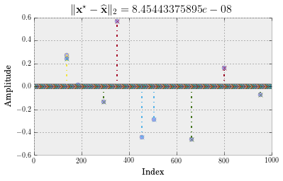
This is great! IHT finds $\mathbf{x}^\star$ fast and ‘accurately’. How fast? Let’s create a convergence plot.
# Plot
plt.rc('text', usetex=True)
plt.rc('font', family='serif')

xs = range(len(x_list))
plt.plot(xs, x_list, '-o', color = '#3399FF', linewidth = 4, alpha = 0.7, markerfacecolor = 'b')
plt.yscale('log')
plt.xlabel(r'\text{Iterations}')
plt.ylabel(r"$\|\mathbf{x}^\star - \widehat{\mathbf{x}}\|_2$")

# Make room for the ridiculously large title.
plt.subplots_adjust(top=0.8)
plt.show()
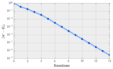
It turns out that vanilla IHT converges to $\mathbf{x}^\star$ linearly, according to the following theorem (for convergence in function values):
Theorem 1 (Convergence of IHT in function values) [7]. Suppose $\mathbf{x}^\star$ is an $k$-sparse vector satisfying $\mathbf{y} = \boldsymbol{\Phi} \mathbf{x}^\star$ and the isometry constants of the matrix $\boldsymbol{\Phi}$ satisfies $\delta_{2k} < 1/3$. Then, IHT computes an s-sparse vector $\widehat{\mathbf{x}} \in \mathbb{R}^p$ such that $||\mathbf{y} - \boldsymbol{\Phi} \widehat{\mathbf{x}}||_2 \leq \epsilon$ in \(\Bigg\lceil \frac{1}{\log\left(\tfrac{1 − \delta\_{2k}}{2\cdot \delta\_{2k}}\right)} \cdot \log \left(\frac{\|\|\mathbf{y}\|\|\_2 ^2}{\epsilon}\right) \Bigg\rceil\) iterations.
…(remark: this holds for step size different than 1 - we will get back to that in the next pot) and according to the following theorem (for convergence in estimates):
Theorem 2 (Convergence of IHT in estimates) [8]. Given observations $\mathbf{y} = \boldsymbol{\Phi} \mathbf{x}^\star$, where $\mathbf{x}^\star$ is $k$-sparse. If $\boldsymbol{\Phi}$ satisfies the RIP with $\delta_{3k} < 1/15$, then, IHT recovers $\widehat{\mathbf{x}}$ such that \(\|\|\mathbf{x}^\star - \widehat{\mathbf{x}}\|\|\_2 \leq 2^{-i} \|\|\mathbf{x}^\star - \mathbf{x}\_0\|\|\_2,\) after $i$ iterations.
In the next post:
- We will discuss further the properties of vanilla IHT.
- We will briefly describe constant step size selections that lead to several IHT variants.
References
[1] Emmanuel Candès, Compressive Sampling, Int. Congress of Mathematics, 3, pp. 1433-1452, Madrid, Spain, 2006.
[2] Richard Baraniuk, Compressive sensing, IEEE Signal Processing Magazine, 24(4), pp. 118-121, July 2007.
[3] Emmanuel Candès and Michael Wakin, An introduction to compressive sampling, IEEE Signal Processing Magazine, 25(2), pp. 21 - 30, March 2008.
[4] Ingrid Daubechies, Ten Lectures on Wavelets, Society for Industrial and Applied Mathematics, 1992.
[5] Stéphane Mallat, A wavelet tour of signal processing, 2nd Edition, Academic Press, 1999.
[6] Roman Vershynin, Introduction to the non-asymptotic analysis of random matrices, Chapter 5 in Compressed Sensing, Theory and Applications, edited by Y. Eldar and G. Kutyniok, Cambridge University Press, 2012. pp. 210–268.
[7] Rahul Garg, and Rohit Khandekar, Gradient descent with sparsification: An iterative algorithm for sparse recovery with restricted isometry property, in ICML, 2009.
[8] Thomas Blumensath, Mike Davies, Iterative hard thresholding for compressed sensing, Applied and Computational Harmonic Analysis, vol. 27, no. 3, pp. 265-274, 2009.