The AdaGrad algorithm

In this note, I briefly describe the main points of the AdaGrad algorithm.

Disclaimer: These notes assume that the reader can build up the story by just looking into the mathematical expressions.

Problem setting

The original Adagrad algorithm was designed for convex objectives with an empirical loss form:

For simplicity, we have removed any constraints on $x$, and we assume $f_i(\cdot)$ are differentiable with gradient $\nabla f_i(x)$.

Gradient descent (GD) follows the recursion:

and stochastic gradient descent (SGD) satisfies:

where the difference lies in the gradient calculation (i.e., using all $f_i(\cdot)$ or a subset of them).

Using preconditioners in gradient descent

Another method, that is usually deprecated due to its increased computational complexity, is Newton’s method. Newton’s method favors a much faster convergence rate (number of iterations) at the cost of being more expensive per iteration (trade-off). For convex problems, the recursion is similar to GD:

where $\eta$ is often close to one (damped-Newton) or one, and $H^{-1}$ denotes the Hessian of $F$ at the current point.

The above suggest a general rule in optimization: find any preconditioner (in convex optimization it has to be positive semi-definite) that improves –at least in practice– the performance of gradient descent (in terms of iterations to get to an $\varepsilon$-close solution), but without wasting too much “energy” to compute that precoditioner. The above result into:

where preconditioner = $B$.

These ideas date back to 50’s; look for the DFP method, the BFGS method and the Dennis and More analysis.

The AdaGrad variation

The AdaGrad algorithm is just a variant of preconditioned stochastic gradient descent, where $B$ is cleverly selected and updated regularly, and the gradient calculation follows SGD.

In particular, $B_t$ is selected to be a diagonal preconditioner matrix and is updated using the stochastic gradient information, as follows:

i.e., it is the diagonal approximation of the inverse of the square roots of gradient outer products, until the $t$-th iteration. This way we obtain different weights for each variable component (that’s why we have the $\texttt{diag}(\cdot)$ part), and hopefully we can keep the step size $\eta$ constant.

The above lead to the recursion:

where $(B_t)_{jj}$ is when we focus only the diagonal elements of the matrix.

Practical variant

In order to avoid divisions with zeros, one adds a very small quantity $\zeta > 0$ in the denominator (with a slight abuse of notation):

Some experiments

Recently, I started revisiting the zoo of neural network training algorithms (that’s the reason of this post: to have it reminding me the performance of each algorithm). I will follow both a “modern” and an “ancient” point of view of comparing algorithm. Which are these algorithms and what I mean by “modern and “ancient”?

“Modern” and “ancient” point of view

Let me start reverse-wise and explain what I mean by “ancient” point of view.

Machine learning has evolved over the past 2 decades with great pace, so that many things have been (re)invented and changed: Theory became stronger and wider, new algorithms have been developed, and new problem settings have emerged.

The “modern” vs. “ancient” point of view has to do with the last part. Writing a paper with just linear regression as an application was ok for research a decade ago: one could get in NIPS/ICML with some theory + algorithms, and with experiments on real data and boilerplate ordinary least-squares objectives. Nowadays, any paper that just has least-squares experiments most probably is going to be criticized as weak since this does not “…mirror current advances and real-world problems”. The last part implies in most cases that it is just not neural networks.

Nevertheless, here, I will follow both “ancient” and “modern” routes: I will use linear/logistic regression to compare some of the recent algorithms used in neural networks, since we have to understand the strengths and weaknesses of each algorithm, even for simple settings. Later on, I will consider simple settings of neural networks and apply the same algorithms there.

Well-conditioned linear regression

Let $x^\star$ be the unknown vector in $\mathbb{R}^p$, assuming $|| x^\star ||_2 = 1$. In standard linear regression, we observe $x^\star$ via the linear mapping:

where $A \in \mathbb{R}^{n \times p}$ is the set of features, and $w \in \mathbb{R}^n$ is an additive noise term. For simplicity we can assume that $w$ is i.i.d. according to a Gaussian distribution, with mean zero and standard deviation $\sigma$.

Given the above, the problem we want to solve is:

for $a_i^\top$ being the rows of the matrix $A$.

It is well known that a key component for characterizing the convergence of an algorithm on such problems is the condition number $\kappa(F)$ of the problem. By definition, the condition number is the ratio:

Here, $L$ is the Lipschitz gradient constant of $F$ and $\mu$ its strong convexity parameter (afterall, we are still in the convex world). The largest the condition number, the harder (=more number of iterations to get a specific error tolerance $|| \widehat{x} - x^\star ||_2 \leq \varepsilon$ ) the problem is. For the case of least squares, the condition number of the problem is proportional to the condition number of $A^\top A$:

The setting is given in the code below - it is written in Maltab (another deprecated choice but personally I believe Matlab is still at the top of the list for algorithmic protoyping…).

%% Problem setting

% Dimension
p = 50;								

% Number of measurements
n = 200;							

% Noise std
sigma = 1e-3;						

% This will vary below.
kappa = 10^2;						

log_smin = -1;
log_smax = log10(sqrt(kappa) * 10^log_smin);

% Measurement matrix
A = 1/sqrt(n) * randn(n, p); 		
[U, ~, V] = svd(A, 'econ');

% Force condition number be kappa
S = logspace(log_smin, log_smax, p);
S = S(end:-1:1);					

A = U * diag(S) * V';

% Ground truth
x_star = randn(p, 1);				
x_star = x_star./norm(x_star);

% Noise
w = randn(n, 1);					
w = sigma * w./norm(w); 

% Measurements in y
y = A*x_star + w;					

• AdaDelta vs. AdaGrad vs. plain Gradient Descent with step size $\tfrac{1}{L}$.

For gradient descent, we use the recursion:

and we compare it to:

where $\zeta$ is set to a small number (say, $10^{-10}$).

The result looks something like this:

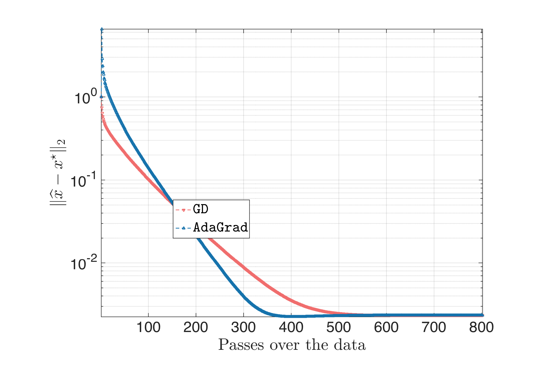
Both algorithms start at the same all-zero starting point; AdaGrad diverges the first couple of iterations, but then it “covers” quickly the lost ground. There are also cases that plain gradient descent is slightly better than AdaGrad, but overall with this step size, $\text{AdaGrad} > \text{Gradient Descent}$.

• AdaGrad vs. plain Gradient Descent with step size $\eta = 0.1$.

Selecting step size is one of the most important subroutines in optimization. Claiming that one algorithm is better than another, for a given problem, is a very strong statement: we need to push the boundaries of $\eta$ values, until the point the algorithm starts “harming” itself, and pick that step size as the step size for comparison. Each algorithm has a different range of $\eta$ values that best works for them. However, since this is often an expensive search, people rely on standard selected step sizes, such as $\eta = 0.1$.

The result looks something like this:

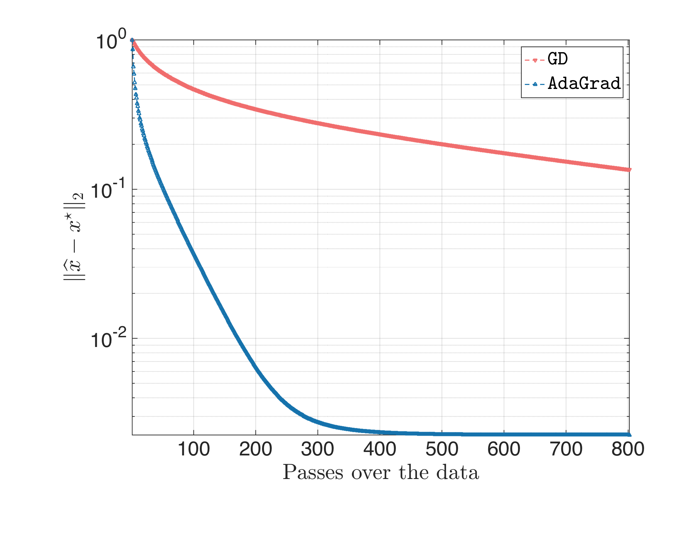
This also justifies that AdaGrad is kind-of immune to the $\eta$ selection: after a few iterations, the weights from the gradient calculation in $B$ pay-off.

• AdaGrad vs. plain Gradient Descent with carefully selected step size.

But, what if we jack up the step size a bit, to find the boundaries of the algorithms. For this particular setting, step size $\eta = 1.9$ works pretty well for gradient descent; step size $\eta \in [0.1, 0.2] $ also works the best for AdaGrad. The result is as follows:

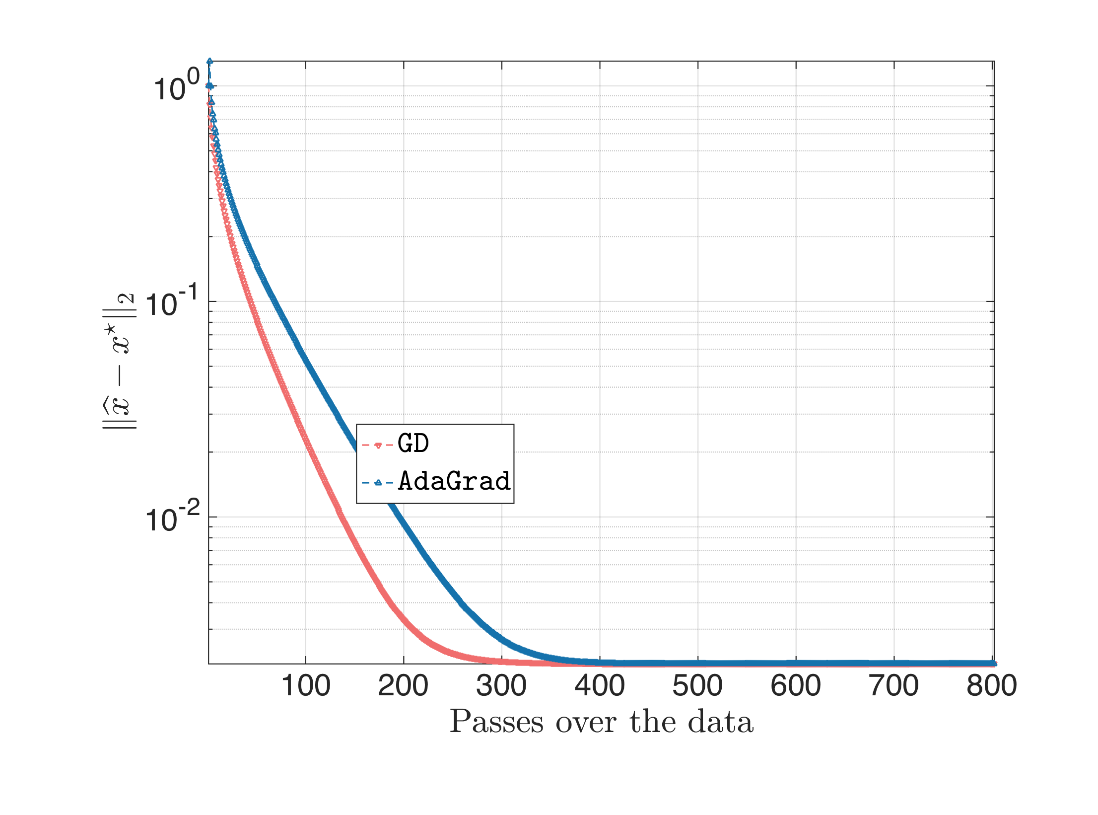
I.e., the secret sauce of AdaGrad is not on necessarily accelerating gradient descent with a better step size selection, but making gradient descent more stable to not-so-good $\eta$ choices. It is important to remember that both plain gradient descent and AdaGrad use the same information per iteration (i.e., the gradient information), which further means that practically there is a step size in gradient descent that can make it (more or less) the same efficient to AdaGrad.

Ill-conditioned linear regression

Let us repeat the above experiment for $\kappa(A^\top A)$ much larger.

% New condition number
kappa = 10^6;						

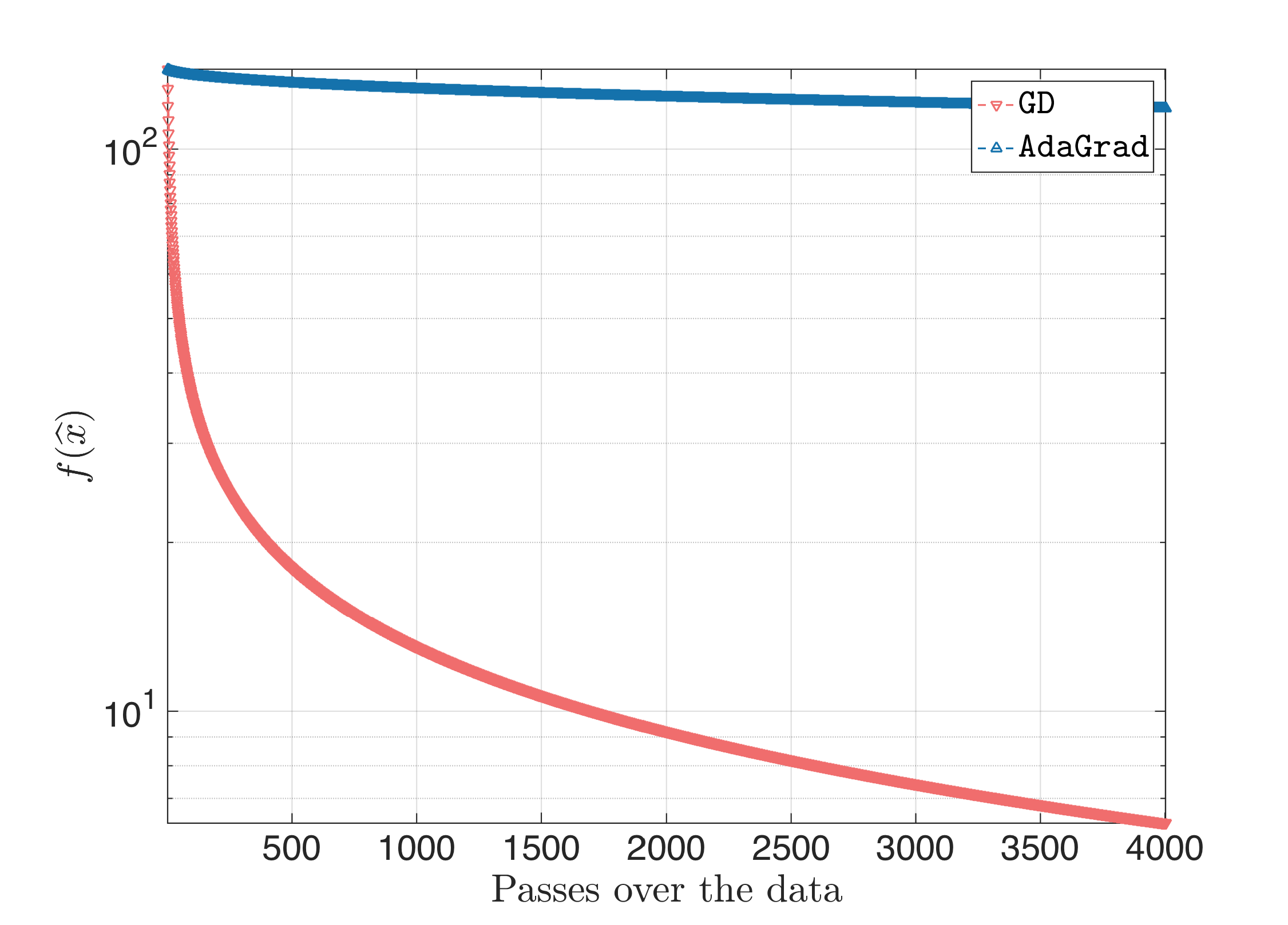
Following the same steps, for $\eta = \frac{1}{L}$ we get:

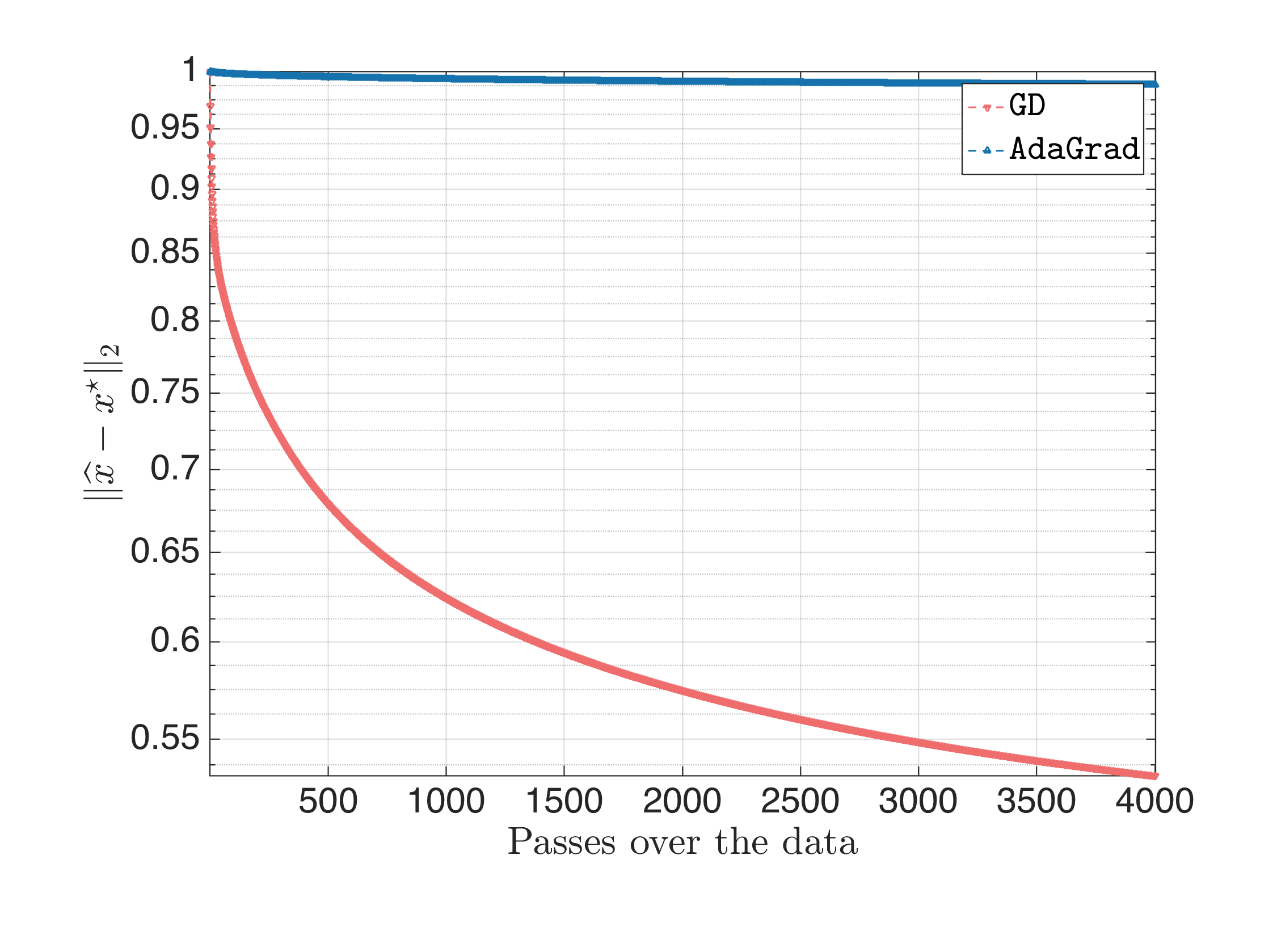
For $\eta = 0.1$, we get:

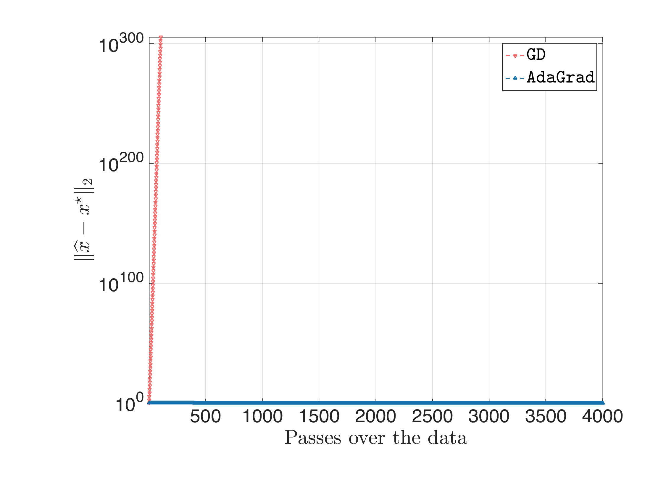
where Gradient Descent diverges (and this is expected since guaranteed convergence is attained if the step size is less than $\approx \frac{2}{L} \approx 2 \cdot 10^{-4}$); and finally:

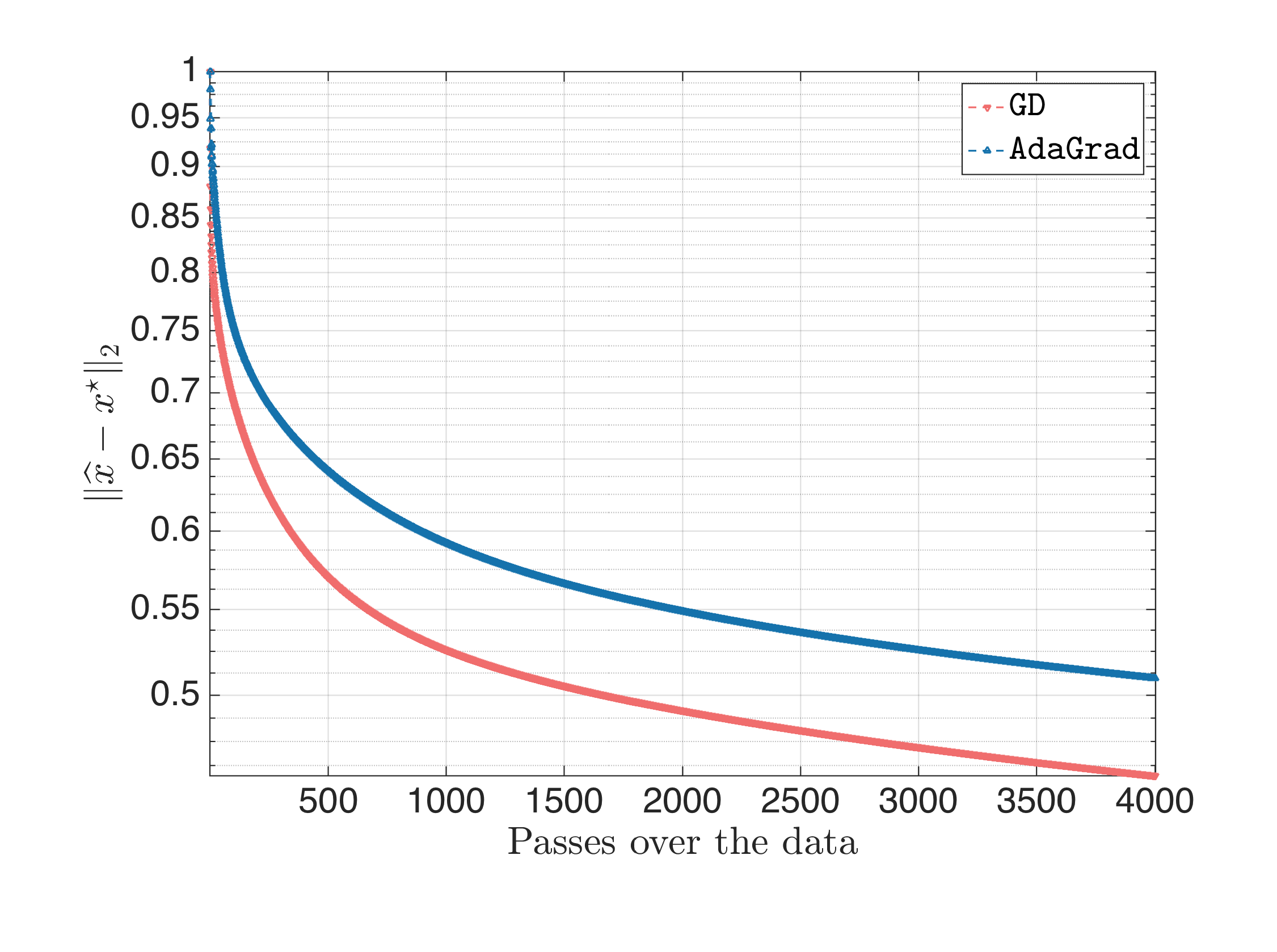
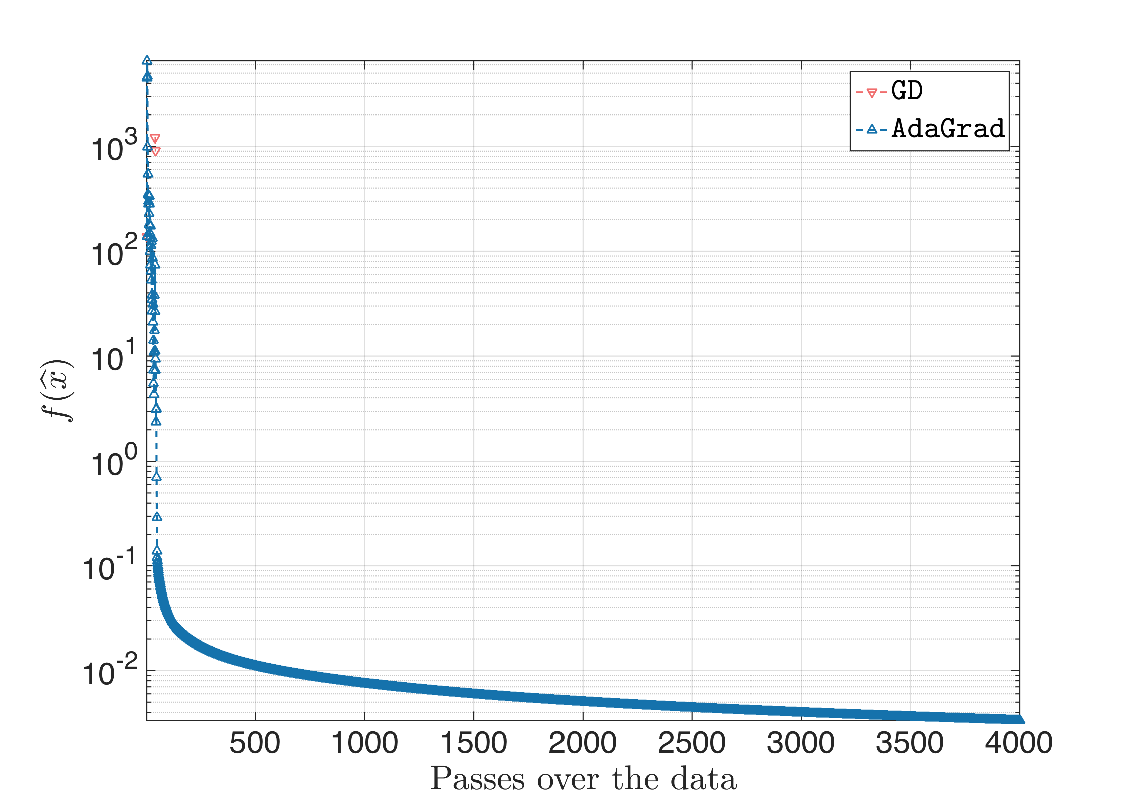
for carefully selected step sizes. In the last part, I want to stress out that, for ill-conditioned problems, AdaGrad is not that “immune” of the $\eta$ selection: various $\eta$’s lead to various behaviors, with most of them being inferior of gradient descent, and few of them leading to superior performance.

Logistic regression

So far, we considered a convex –both having Lipschitz continuous gradients and being strongly convex– problem. A less strict class of functions is that of problems that just satisfy the Lipschitz gradient continuity: dropping strong convexity by itself is (was?) enough to generate a new set of research papers where the algorithms remain more or less the same, but the theory had to change, since we cannot use any more the nice properties of strong convexity. A more important consequence is that usually one has to be content with slower rates (it is the difference between sublinear and linear convergence rates).

Let us now compare AdaGrad with Gradient Descent in such a setting. The most classical scenario is that of logistic regression: instead of regressing with real values (this is what we do in least-squares: we try to find the solution to a linear problem, by not restricting the output $y$), we have binary or multi-valued outputs, in order to model well the task of classification.

Consider the following setting: let $x^\star$ be the unknown vector in $\mathbb{R}^p$, assuming $|| x^\star ||_2 = 1$. In our simplistic logistic regression setting, we observe $x^\star$ via the sequence of linear + non-linear mappings:

where $A \in \mathbb{R}^{n \times p}$ is the set of features, and $w \in \mathbb{R}^n$ is an additive noise term. Observe that we no longer observe the output of the linear system per-se: we observe only the signs of that operation, modeling in a way the classication problem of two classes.

One way to model this problem in math is by using the logistic function. Thus:

for $a_i^\top$ being the rows of the matrix $A$, and $b$ being the bias term.

Globally, over the whole domain, logistic function as defined above has strong convexity paramter $\mu(F) := \mu = 0$. Thus, the condition number of the function in this case is not well-defined. Nevertheless, the condition number of $A^\top A$ still plays important role in the behavior of the algorithms: the bigger the condition number, the more difficult the problem is.

The setting is given in the code below.

%% Problem setting

% Dimension
p = 50;								

% Number of measurements
n = 200;							

% Noise std
sigma = 1e-3;						

% This will vary below.
kappa = 10^2;						

log_smin = -1;
log_smax = log10(sqrt(kappa) * 10^log_smin);

% Measurement matrix
A = 1/sqrt(n) * randn(n, p); 		
[U, ~, V] = svd(A, 'econ');

% Force condition number be kappa
S = logspace(log_smin, log_smax, p);
S = S(end:-1:1);					

A = U * diag(S) * V';

% Ground truth
x_star = randn(p, 1);				
x_star = x_star./norm(x_star);

% Bias vector
b = randn(n, 1);                     
b = 0.1 * b./norm(b); 

% Noise
w = randn(n, 1);					
w = sigma * w./norm(w); 

% Measurements in y
y = sign(A*x_star + b + w); 				

• AdaGrad vs. plain Gradient Descent with step size $\tfrac{1}{L}$.

The story is the same. For gradient descent, we use the recursion:

and we compare it to:

where $\zeta$ is set to a small number (say, $10^{-10}$).

The result looks something like this:

Both algorithms start at the same all-zero starting point; overall with this step size, in this setting $\text{AdaGrad} < \text{Gradient Descent}$.

• AdaGrad vs. plain Gradient Descent with carefully selected step size.

For a wide range of values (I tried $\eta \in [1, 40]$), the result looks something like this, where as the step size increases, AdaGrad catches-up the performance of Gradient Descent:

One can say that AdaGrad and Gradient Descent perform similarly for these cases.

Repeating the above experiment for $\kappa(A^\top A)$ much larger:

% New condition number
kappa = 10^6;						

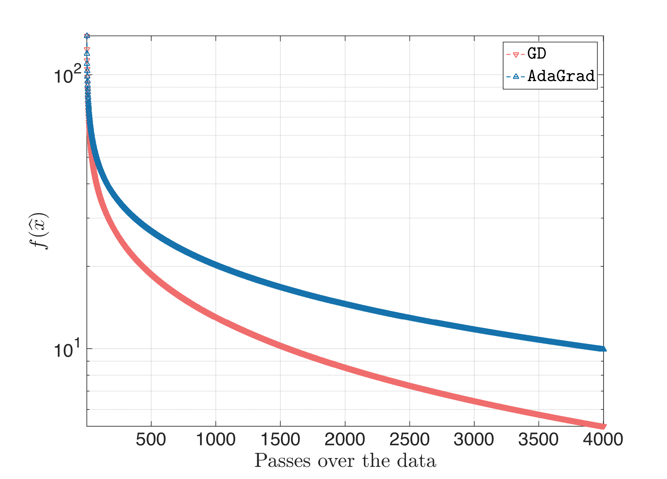
we get for $\eta = \frac{1}{L}$:

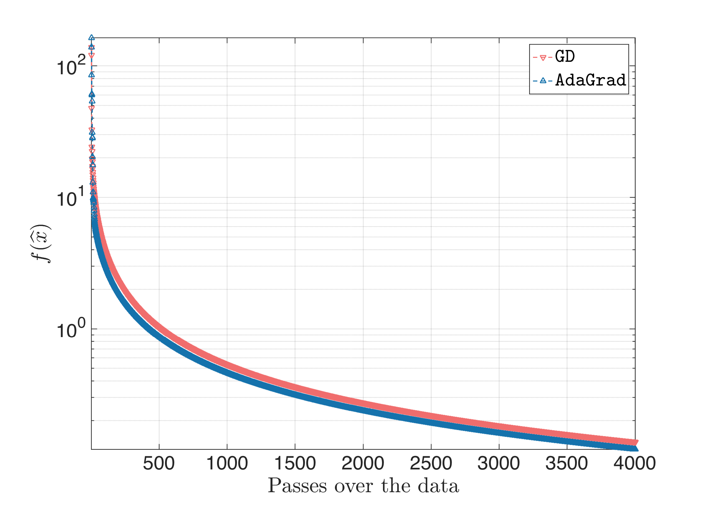
When we start jacking-up the step size, Gradient Desccent stops being superior to AdaGrad: the latter better approximates the ill-curvature of the problem, and performs better (the following plot is for $\eta = 10$ and the same behavior is observed when we keep increasing $\eta$):

Feedforward Neural Network (FNN) training - MNIST

Here, we consider a small feed forward neural network arcitecture. The task is the classical MNIST classification problem. The setting is pretty much well-known and standard (specs of dataset, size of training/validation/testing sets, etc.), so we will skip that part; for more information see here.

The network architecture includes three hidden layers with ReLU activation functions.

• The input is $ 28 \times 28 $ images of digits in the range ${0, \dots, 9}$. As usual, we flatten out the inputs into a $784$-dimensional vector.
• The first layer takes as input $784$-dimensional vectors (say, $\beta \in \mathbb{R}^{784}$), multiplies it with a variable weight vector $W_1$ of dimension $784 \times 384$ (say, $W_1 \in \mathbb{R}^{384 \times 784}$), and adds a variable bias term of size $384$ (say, $b_1 \in \mathbb{R}^{384}$). Finally, the result is passed through a entry-wise ReLU function $g_1: \mathbb{R}^{384} \rightarrow \mathbb{R}^{384}$ such that:

        Alltogether this leads to:

• The second layer is no different than the first layer: the input is the $384$-dimensional vector created in the previous layer, the output is further squeezed to a $256$-dimensional vector. The idea is similar: we define a –different– variable weight matrix $W_2 \in \mathbb{R}^{256 \times 384}$, a –different– variable bias variable $b_2 \in \mathbb{R}^{256}$, and the final output satisfies:

        Observe that $g_1$ is identical to $g_2$, but now we have a different sized input vector.

• The third layer is similar to the above: The input is a $256$-dimensional vector, the output is a $10$-dimensional vector (= number of classes to classify). We define again a -different– variable weight vector $W_3 \in \mathbb{R}^{10 \times 256}$ and a –different– variable bias vector $b_3 \in \mathbb{R}^{10}$. The final layer includes no ReLU functions, but the output is passed through a softmax function. The softmax function operates as a probability distribution “creator”, giving highest probabilities to the largest entries of the $10$-dimensional vector:

The final objective over the unknown variables $x := {W_1, W_2, W_3, b_1, b_2, b_3}$ is the cross-entropy objective. In particular, denoting our dataset with $\beta_i$s (these are the $n$ training images), and the corresponding labels with $y_i$s (these are encoded as $10$-dimensional, one-hot vectors, with $1$ at the corresponding class, and the rest zero), we have:

Given the above simplistic network, and its objective, we test the efficiency of AdaGrad versus:

• Plain stochastic gradient descent with constant step size:

• Stochastic gradient descent with Nesterov momentum:

and for settings where:

• The batch size (i.e., we talked above for a single input $\beta \in \mathbb{R}^{784}$; now think of an input of size $\mathbb{R}^{784 \times B}$, where $B$ is the batch size). We consider $B = 1000$ (relatively small batch size) and $B = 50000$ (full batch). We also plot the case of SGD with a small batch size $B = 50$.
• The step size is set constant to $\eta = 0.25$ for AdaGrad, $\eta = 0.25$ for SGD with Nesterov momentum, and $\eta = 0.5$ for SGD. These values were selected after checking several values for this hyperparameter. We try not to be conservative (thereby, the increased step size compared to the classical $\eta = 0.1$); at the same time, we want a relatively stable performance over different realizations.
• By realizations, we mean mostly the initialization of parameters, as well as the randomness of shuffling the input dataset. For the former, we use standard random initialization (using truncated normal distributions).
• We use no other regularization techniques. Our purpose is to test algorithms on the simplest objective scenaria to understand their power; thus, we are not interested in state of the art test error performance.

The results look like the following; the same behavior has been observed over several runs of the same code. The vertical axis represents accuracy error on the training/validation set; the horizontal axis shows the actual gradient calculations required.

The algorithms are encoded as:

• AdaGrad2: $B = 1000$
• AdaGrad3: $B = 50000$
• Nesterov2: $B = 1000$
• Nesterov3: $B = 50000$
• SGD1: $B = 50$
• SGD2: $B = 1000$
• (Neglect SGD1/.)

Some comments:

• SGD and SGD with momentum seems to work quite efficiently without adaptive techniques: constant step size, and classic routines for momentum seem to be robust. We will continue working along these lines in the future posts also.
• Adagrad has a good performance; nevertheless, there is no clear advantage compared to SGD2, when we set $B = 1000$ for both cases.
• We observe that large batch training can be beneficial: while AdaGrad3 has a slow convergence, Nesterov3 seems to achieve a very good performance: while slower, it is more stable (there are no blurred “ups-downs” - remember the plot is smoothed). On the contrary, methods with smaller batches have a lot of “jumps”.
• Introducing momentum in Adagrad might be interesting; this will lead us to algorithms like Adam and RMSProp.