Introduction to quantum computing: From classical to quantum (part II).

Sources:

“Quantum computing for computer scientists”, N. Yanofsky and M. Mannucci, Cambridge Press, 2008.

“The Feynman Lectures on Physics”, R. Feynman, R. Leighton, M. Sands, Volume III, 1963.

This is part of a (probably) long list of posts regarding quantum computing. In this post, we discuss the part II of the post where we take the leap from classical to quantum notions.

Disclaimer: while the material below might seem too simple for some scientists, I suggest not skimming over this post - personally, I always enjoy reading something that I believe I own, as επαναληψη μητηρ πασης μαθησεως (repetition is the mother of any knowledge)

This post follows the perspective in Feynman’s lecture:

“We cannot make the mystery go away by “explaining” how it works. We will just tell you how it works. In telling you how it works we will have told you about the basic peculiarities of all quantum mechanics.”

The double-slit experiment - simplified version

Here, we will describe a simplified version of the double-slit experiment - we will make an effort to describe the physical phenomenon of the double-slit experiment later on in the text.

Macroscopic world: The archery analog

Let us make the following hypothetical scenario. An archer throws arrows over a wall with two slits that are far apart. Behind the wall there are five targets, all of them in a row along the wall. However, the arrow, given that passes through one of the slits, can hit at most 3 targets; one of the target is reachable through both slits.

The above can be described via the following transition diagram.

Here, node 0 is where the archer is; nodes 1 and 2 are the two slits on the wall (the archer every time passes an arrow through the slits - which slit is not certain but has 50% possibility); nodes 3-7 are the targets, with assigned probabilities that the arrow will end on each target.

Observe that node 5 can get hit in one of two ways: from the top slit going down or from the bottom slit going up.

In this simplistic scenario, it is assumed that the arrow takes a single time click to get from the archer to the wall, and another time click to travel from the slit to the targets.

Let us compute the transition matrix $\mathbf{P}$:

\[\mathbf{P} = \begin{bmatrix} 0 & 0 & 0 & 0 & 0 & 0 & 0 & 0 \\ \tfrac{1}{2} & 0 & 0 & 0 & 0 & 0 & 0 & 0 \\ \tfrac{1}{2} & 0 & 0 & 0 & 0 & 0 & 0 & 0 \\ 0 & \tfrac{1}{3} & 0 & 1 & 0 & 0 & 0 & 0 \\ 0 & \tfrac{1}{3} & 0 & 0 & 1 & 0 & 0 & 0 \\ 0 & \tfrac{1}{3} & \tfrac{1}{3} & 0 & 0 & 1 & 0 & 0 \\ 0 & 0 & \tfrac{1}{3} & 0 & 0 & 0 & 1 & 0 \\ 0 & 0 & \tfrac{1}{3} & 0 & 0 & 0 & 0 & 1 \end{bmatrix}\]

The above transition matrix models the behavior of the arrow for one time click. Focus on the columns of the matrix, and puts labels 0 to 7. E.g., the first column models the fact that we are on the archer node and there are 50% probability the archer will lead to nodes 1 and 2 (the two slits).

The transition matrix after two time clicks satisfies:

\[\mathbf{P}^2 = \begin{bmatrix} 0 & 0 & 0 & 0 & 0 & 0 & 0 & 0 \\ 0 & 0 & 0 & 0 & 0 & 0 & 0 & 0 \\ 0 & 0 & 0 & 0 & 0 & 0 & 0 & 0 \\ \tfrac{1}{6} & \tfrac{1}{3} & 0 & 1 & 0 & 0 & 0 & 0 \\ \tfrac{1}{6} & \tfrac{1}{3} & 0 & 0 & 1 & 0 & 0 & 0 \\ \tfrac{1}{3} & \tfrac{1}{3} & \tfrac{1}{3} & 0 & 0 & 1 & 0 & 0 \\ \tfrac{1}{6} & 0 & \tfrac{1}{3} & 0 & 0 & 0 & 1 & 0 \\ \tfrac{1}{6} & 0 & \tfrac{1}{3} & 0 & 0 & 0 & 0 & 1 \end{bmatrix}\]

Thus, starting with the state vector $x = \left[1 ~0 ~0 ~0 ~0 ~0 ~0 ~0\right]^\top$, we compute:

\[\mathbf{P}^2 \mathbf{x} = \left[0 ~0 ~0 ~\tfrac{1}{6} ~\tfrac{1}{6} ~\tfrac{1}{3} ~\tfrac{1}{6} ~\tfrac{1}{6}\right]^\top\]

Important observation for our discussion below is that the arrow might get to the node 5 with probability $\tfrac{1}{3}$: half comes from the positibility the arrow to pass the upper slit and the other half from the lower slit.

Microscopic world: The photon analog

Let us re-describe the experiment in the microspopic world. Instead of archers and arrows, we have a photon generator and photon packets. The experiment is very similar, where we still have two slits on a wall and (abstractly) 5 detectors behind the wall.

The major change we will make is the transition probabilities from one node to the other: we will assume that the probabilities are computed as the modulus of complex numbers. The graph is as follows:

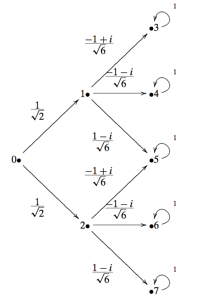
As an example, the modulus squared of $\tfrac{1}{\sqrt{2}}$ is $\tfrac{1}{2}$, which corresponds to the fact that there is half probability that the photon will pass through either slit. Similarly, one can figure out what the other “probabilities” correspond to.

The transition matrix of this graph is:

\[\mathbf{P} = \begin{bmatrix} 0 & 0 & 0 & 0 & 0 & 0 & 0 & 0 \\ \tfrac{1}{\sqrt{2}} & 0 & 0 & 0 & 0 & 0 & 0 & 0 \\ \tfrac{1}{\sqrt{2}} & 0 & 0 & 0 & 0 & 0 & 0 & 0 \\ 0 & \tfrac{-1+i}{\sqrt{6}} & 0 & 1 & 0 & 0 & 0 & 0 \\ 0 & \tfrac{-1-i}{\sqrt{6}} & 0 & 0 & 1 & 0 & 0 & 0 \\ 0 & \tfrac{1-i}{\sqrt{6}} & \tfrac{-1+i}{\sqrt{6}} & 0 & 0 & 1 & 0 & 0 \\ 0 & 0 & \tfrac{-1-i}{\sqrt{6}} & 0 & 0 & 0 & 1 & 0 \\ 0 & 0 & \tfrac{1-i}{\sqrt{6}} & 0 & 0 & 0 & 0 & 1 \end{bmatrix}\]

Computing the probabilities of two consecutive time clicks leads to:

\[|\mathbf{P}^2|^2 = \begin{bmatrix} 0 & 0 & 0 & 0 & 0 & 0 & 0 & 0 \\ 0 & 0 & 0 & 0 & 0 & 0 & 0 & 0 \\ 0 & 0 & 0 & 0 & 0 & 0 & 0 & 0 \\ \tfrac{1}{6} & \tfrac{1}{3} & 0 & 1 & 0 & 0 & 0 & 0 \\ \tfrac{1}{6} & \tfrac{1}{3} & 0 & 0 & 1 & 0 & 0 & 0 \\ 0 & \tfrac{1}{3} & \tfrac{1}{3} & 0 & 0 & 1 & 0 & 0 \\ \tfrac{1}{6} & 0 & \tfrac{1}{3} & 0 & 0 & 0 & 1 & 0 \\ \tfrac{1}{6} & 0 & \tfrac{1}{3} & 0 & 0 & 0 & 0 & 1 \end{bmatrix}\]

These transition probabilities are almost the same with the experiment in the macroscopic world. However, there is a distinct difference: The probability of a photon to end to the node 5 is actually 0! To see this, let us first add the probabilities:

\[\tfrac{1}{\sqrt{2}} \left(\tfrac{-1+i}{\sqrt{6}} \right) + \tfrac{1}{\sqrt{2}}\left(\tfrac{1-i}{\sqrt{6}} \right) = \tfrac{-1 + i + 1 -i}{\sqrt{12}} = 0\]

Thus, taking the modulus of (complex) zero leads to zero probability. The macroscopic interpretation of the position of the photon is not entirely adequate. From our description it seems that the photon passes through both slits at the same time (even if a single photon is sent!) and when it exits both slits, it cancels itself out at node 5. A photon is not in a single position, rather it is in many positions, a superposition.

This example shows one distinct difference between dynamics with real numbers and dynamics with complex numbers!

Quoting Yanofsky and Mannucci:

This might generate some justifiable disbelief. Afterall, we do not see things in many different positions. Our everyday experience tells us that things are in one position or (exclusive or!) another. How can this be? The reason we see particles in one particular position is because we have performed a measurement. When we measure something at the quantum level, the quantum object that we have measured is no longer in a superposition of states, rather it collapses to a single classical state. So we have to redefine what the state of a quantum system is: a system is in state $\mathbf{x}$ means that after measuring it, it will be found in position $i$ with probability equal to the modulus squared.

It is exactly this superposition of states that is the real power behind quantum computing. Classical computers are in one state at every moment. Imagine putting a computer in many different classical states simultaneously and then processing with all the states at once. This is the ultimate in parallel processing! Such a computer can only be conceived of in the quantum world.

Some links about the true double-slit experiment

I strongly recommend watching the PBS video on double-slit experiment and what it means.