Introduction to quantum computing: Basic quantum theory.

Sources:

“Quantum computing for computer scientists”, N. Yanofsky and M. Mannucci, Cambridge Press, 2008.

This is part of a (probably) long list of posts regarding quantum computing. In this post, we will talk about quantum states, observables, what it means to measure a quantum state, and the dynamics of quantum states.

Disclaimer I: while the material below might seem too simple for some scientists, I suggest not skimming over this post - personally, I always enjoy reading something that I believe I own, as επαναληψη μητηρ πασης μαθησεως (repetition is the mother of any knowledge)

Disclaimer II: reading this post might leave you with more questions than answers. We will revisit the notions in this post in our future posts.

Quantum states

Let us introduce the following simplistic scenario. Consider a line with discrete points as possible positions of particles. See for example:

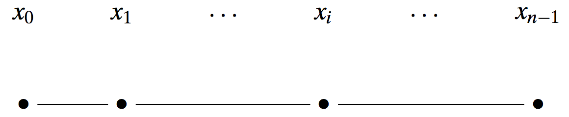
Each position (bold dot) on the line corresponds to a state of the particle (let’s say that the particle “lies” in one/some of these states). The particple being in state $\mathbf{x}_i$ is going to be denoted with the Dirac ket notation (no worries, it is nothing but a different way to define vectors in space): $|\mathbf{x}_i \rangle$. Moreover, let us make the following association of states with vectors in the $n$-dimensional space (remember, we have $n$ states):

\[|\mathbf{x}_0 \rangle \longrightarrow \left[1 ~0 ~\dots ~0\right]^\top \\ |\mathbf{x}_1 \rangle \longrightarrow \left[0 ~1 ~\dots ~0\right]^\top \\ \vdots \\ |\mathbf{x}_{n-1} \rangle \longrightarrow \left[0 ~0 ~\dots ~1\right]^\top\]

From the classical mechanics perspective, this is what we all need in order to explain a “system” like the above: we can characterize in the macroscopic world the state where the particle lies exactly, by observing it! However, the same does not hold for the microscopic quantum world: we need to define all posible combinations of states as possible states!

In particular, let $| \mathbf{\psi} \rangle $ be an arbitrary state, that can be described as a linear combination of all the above states. For suitable known complex weights $c_0, c_1, \dots, c_{n-1}$, $| \mathbf{\psi} \rangle$ can be written as:

\[| \mathbf{\psi} \rangle = c_0 |\mathbf{x}_0 \rangle + c_1 |\mathbf{x}_1 \rangle + \dots + c_{n-1} |\mathbf{x}_{n-1} \rangle.\]

In this case, given that we know the “basis” w.r.t. $\mathbf{x}_i$’s, we can represent the state $|\mathbf{\psi} \rangle$ by just knowing the coefficients $c_i$. This state is in superposition of all the basic states $| \mathbf{x}_i \rangle$. You can say that $| \mathbf{\psi} \rangle$ lies on all states simultaneously; however, when we observe it, the state will collapse to one of the basic states. Which state? The one selected with probability $\tfrac{|c_i|^2}{| | \mathbf{\psi} \rangle |_2}$, for some $i$. In other words, the (normalized) modulus squares of the complex numbers $c_i$ play the role of the probabilities of the state being collapsed to that basic state.

It is basic to remember that by the time we observe $| \mathbf{\psi} \rangle$, it collapses to that state.

Some facts about the bra-ket notation

The bra-ket notation is (more or less) the quantum-mechanics-way to describe vectors and inner products of vectors. Let $ \langle \mathbf{\varphi} |$ and $| \mathbf{\psi} \rangle $ be two vectors in $\mathbb{C}^n$. The difference between the two vectors is the orientation: $| \mathbf{\psi} \rangle $ is called the ket and represents column vectors; $ \langle \mathbf{\varphi} |$ is called the bra and represents a Hermitian conjugate of a ket, and thus it is a row vector.

The standard notation for inner product in the bra-ket notation is:

\[\langle \mathbf{\varphi} | \mathbf{\psi} \rangle \equiv \left( \langle \mathbf{\varphi} | \right) \cdot \left( | \mathbf{\psi} \rangle \right) \\ = \left[\varphi_1^\dagger ~\varphi_2^\dagger ~\dots~ \varphi_n^\dagger \right] \cdot \begin{bmatrix} \psi_1 \\ \psi_2 \\ \vdots \\ \psi_n \end{bmatrix}.\]

Similarly, the standard notation for the outer product is:

\[| \mathbf{\varphi} \rangle \langle \mathbf{\psi} | \in \mathbb{C}^{n \times n}.\]

Some properties: $\langle \varphi |^\dagger = | \varphi \rangle$ and $| \varphi \rangle^\dagger = \langle \varphi |$; Bras and kets can added: if $| \mathbf{\psi} \rangle = c_0 |\mathbf{x}_0 \rangle + c_1 |\mathbf{x}_1 \rangle + \dots + c_{n-1} |\mathbf{x}_{n-1} \rangle$ $| \mathbf{\psi}’ \rangle = c_0’ |\mathbf{x}_0 \rangle + c_1’ |\mathbf{x}_1 \rangle + \dots + c_{n-1}’ |\mathbf{x}_{n-1} \rangle$, then $| \mathbf{\psi} \rangle + | \mathbf{\psi}’ \rangle = \left(c_0 + c_0’\right) |\mathbf{x}_0 \rangle + \left(c_1 + c_1’\right)|\mathbf{x}_1 \rangle + \dots + \left(c_{n-1} + c_{n-1}’\right)|\mathbf{x}_{n-1} \rangle$; Bras and kets can be multiplied by scalars (not shown here).

Transition amplitudes

To close this chapter, we will introduce the notion of transition amplitudes. Assume we have a collection of kets that form a basis in $\mathbb{C}^n$: e.g., ${ | \mathbf{b}_0 \rangle, \dots, | \mathbf{b}_{n-1} \rangle }$. Then, any ket in $\mathbb{C}^n$ can be written as a linear combination of these basis vectors:

\[|\mathbf{\psi} \rangle = c_0 | \mathbf{b}_0 \rangle + \dots + c_{n-1} |\mathbf{b}_{n-1} \rangle.\]

(In our discussion so far, we used the coordinate bases where $| \mathbf{b}_i \rangle = |\mathbf{x}_i \rangle$, with the latter having 1 in the $i$-th position, and the rest are zeros)

When we observe the state $| \mathbf{\psi} \rangle$, then the following scheme happens:

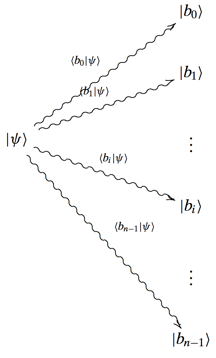
Here, the state, after measuring/observing, ends in any of the basis states $| \mathbf{b}_i \rangle$, where the probability is given by (assuming appropriate normalization): $|c_i|^2$. The transition from $|\mathbf{\psi} \rangle $ to $| \mathbf{b}_i \rangle$ is denoted by the inner product $\langle \mathbf{b}_i | \mathbf{\psi} \rangle$.

To wrap it up:

• We associated a vector to quantum system, through the bra-ket notation.
• States can be superposed.
• The state space has a geometry, associated with an inner product. The likelihood for a given state to transition into another state is measured via the inner product.

Observables

What we have discussed so far is the collection of states a system could be at. Observables correspond to the physical quantities that can be observed in each state of the state space.

Each observable may be thought of as a specific question we pose to the system: assuming it is in state $|\mathbf{\psi} \rangle$, what values/quantities can we possible observe?

An observable corresponds to an linear operator: given a state $| \mathbf{\psi} \rangle \in \mathbb{C}^n$, let us define an observable $\mathbf{\Omega} \in \mathbb{C}^{n \times n}$. The action of the observable is denoted as $\mathbf{\Omega} | \mathbf{\psi} \rangle$ and it is by itself a state.

In quantum mechanics, each observable-linear operator is hermitian. We know that each hermitian matrix has real eigenvalues. Then, the eigenvalues of an observable are the only possible values the observable can take, as a result of measuring it on a given state. In other words, given a state and assuming the observable is seen as a question made, the eigenvalues of the observable are the possible answers.

An example of observables: spin

Given a specific direction in space, in which way is the particle spinning? Define the following three spinning operators:

\[\mathbf{S}_z = \tfrac{h}{2} \cdot \begin{bmatrix} 1 & 0 \\ 0 & -1 \end{bmatrix}\]

for spinning w.r.t. the $z$-direction (up or down),

\[\mathbf{S}_y = \tfrac{h}{2} \cdot \begin{bmatrix} 0 & -j \\ j & 0 \end{bmatrix}\]

for spinning w.r.t. the $y$-direction (in or out),

\[\mathbf{S}_x = \tfrac{h}{2} \cdot \begin{bmatrix} 0 & 1 \\ 1 & 0 \end{bmatrix}\]

for spinning w.r.t. the $x$-direction (left or right). Here, $h$ is the reduced Planck constant; in our discussion, it can be safely ignored. These operators are also known as the Pauli operators and play a key role in quantum state tomography. Each of these matrices are equipped with an orthonormal basis (eigenbasis) and the corresponding eigenvalues (eigenstates).

By definition, for a hermitian matrix $\mathbf{\Omega}$ and a state $| \mathbf{\psi} \rangle$, the quantity $\langle \mathbf{\psi} | \mathbf{\Omega} | \mathbf{\psi} \rangle$ is real. Let us denote this number as: $\langle \mathbf{\Omega} \rangle_{\mathbf{\psi}}$, and it will denote the expected value of observing $\mathbf{\Omega}$ repeatedly on the same state $\mathbf{\psi}$.

Let us conduct an experiment: assume we have a quantum system at a state $|\mathbf{\psi} \rangle$. We want to observe the value of an observable $\mathbf{\Omega}$. Assume the eigenvalues of $\mathbf{\Omega}$: $\lambda_0, \dots, \lambda_{n-1}$. By definition, we will observe one of its eigenvalues. Let us now repeat this experiment $m$ times. At the end of the experiment, we will observe each $\lambda_i$, $p_i$ times, such that $\sum_{i = 1}^n p_i = m$. If we compute:

\[\lambda_0 \tfrac{p_0}{m} + \lambda_1 \tfrac{p_1}{m} + \dots + \lambda_{n-1} \tfrac{p_{n-1}}{m},\]

its value will be very close to $\langle \mathbf{\Omega} \rangle_{\mathbf{\psi}}$ (i.e., a certain frequency distribution on the set of its eigenvalues).

As we defined the mean/expected value of an observable, one can define the variance; while variance lead to the definition of the Heisenberg’s principle, we will leave this part for a future post, if needed.

Measurements

So far, we discussed about asking questions to the system, which are translated as hermitian operators applied on quantum states. The act of measuring is about asking a question and receiving a definite answer (you can see it as building our discussion one module at a time).

So far, through observables, we can only assume that one of the eigenvalues will be the result of an observable (but internally in the system - we never discussed about actually seeing one of these eigenvalues…). Further, even for this case, we are not sure which of the eigenvalues we will observe (we can compute expected values and variances of each observable). Finally, our framework so far does not tell us anything about what happens if we actually observe the eigenvalues.

In contrast to the macroscopic world, quantum systems do get perturbed and modified by the time we measure them. Further, only the probability of observing specific values can be calculated.

It turns out that the following holds: Let $\mathbf{\Omega}$ be an observable and $| \mathbf{\psi} \rangle$ be a state of the system. If the result of measuring $\mathbf{\Omega}$ is its eigenvalue $\lambda$, then the state, after the measurement, has collapsed to the eigenvector of $\mathbf{\Omega}$ that corresponds to the eigenvalue $\lambda$. The probability that we will “land” (as the next state) to the specific eigenvector $|\mathbf{e} \rangle$ is given by $| \langle \mathbf{e}_i | \mathbf{\psi} \rangle |^2$ (i.e, the projection between the two vectors).

To close this section, we would like to note that the order we apply the observables matters. Assume that we are at a state $|\mathbf{\psi} \rangle$ and we ask a specific question (=observable). We get as an answer the eigenvalue $\lambda$. Also, by our discussion so far, the system will collapse to the corresponding eigenvector. Assume now that we re-ask the same question. What would then happen? The answer will still be $\lambda$, since the current state (=eigenvector of the observable) is orthogonal to all eigenvectors, except itself. Now, how do we get out of this state? By asking a different question (=observable). Asking many questions in a different order might lead to different intermediate and final states.

Dynamics of a quantum system

Let us introduce the notion of time in a quantum system, through the sequence of operators we apply to it. We will represent the evolution of a quantum system over time through unitary transformations (Note: could be also hermitian operators; however, we differentiate the notion of observables from the notion of evolution of a quantum system).

Just to give an example: if our system lies at state $|\mathbf{\psi}_t \rangle$ at the time $t$ and at state $|\mathbf{\psi}_{t+1} \rangle$ at the time $t+1$, this transition can be described as:

\[|\mathbf{\psi}_{t+1} \rangle = \mathbf{U} |\mathbf{\psi}_{t} \rangle\]

for some unitary matrix $\mathbf{U}$ with dimensions given by context.

The difference between observables and generic unitary transformations is that the latter satisfy:

• the product of two unitary matrices is always unitary (in any order);
• the inverse of a unitary matrix is unitary.

These proporties are important because they allow “traversing” the quantum system states over time. That is, we can apply sequentially $\mathbf{U}_0 | \mathbf{\psi} \rangle, ~\mathbf{U}_1 \mathbf{U}_0 | \mathbf{\psi} \rangle, \dots, ~\prod_{i = 0}^t \mathbf{U}_i | \mathbf{\psi} \rangle$ to get the evolution. Key property of unitary transformations is that they preserve the energy of the quantum system.

Let us revisit the (very very very) rough description of quantum computing: we start at a state and we apply a sequence of carefully selected unitary transformations that (somehow) reflects the algorithm we want to implement. Then, when we are done, we measure the output to get the final state.

(The discussion of how to select the unitary transformations involve the introduction of the Schrodinger equation. We know that the global energy is preserved in an isolated system, throughout its evolution. Energy is an observable and, for a quantum system, we can use a hermitian matrix to represent it. This matrix is also known as the hamiltonian matrix. Then, the Schrodinger equation describes that the rate of variation from a state to another is proportional to the energy expressed via the hamiltonian matrix. Solving this equation with some initial conditions, we get the evolution.)

In the next post, we will discuss about entanglement and entangled states.