Introduction to quantum computing: Quantum gates.
Sources:
“Quantum computing for computer scientists”, N. Yanofsky and M. Mannucci, Cambridge Press, 2008.
This is part of a (probably) long list of posts regarding quantum computing. In this post, we will talk about the nuts and bolts of quantum computing: quantum gates. For the moment, we will just describe quantum gates in an abstract sense and not relate how these gates are connected to algorithms. But have in mind: even for classical computers, whatever algorithm we design, it needs to be translated to “hardware language”, that further is decomposed as a collection of classic gates.
Disclaimer I: while the material below might seem too simple for some scientists, I suggest not skimming over this post - personally, I always enjoy reading something that I believe I own, as επαναληψη μητηρ πασης μαθησεως (repetition is the mother of any knowledge)
Classical bit
In the macroscopic world, we know that: $(i)$ electricity either passes or not through a circuit, $(ii)$ a proposition is true or false, etc. The above can be easily described through a bit: a bit represents an way to say that we are in a particular state among two states.
There are different ways to represent this information. In this post, we will use the following representation of a bit:
\[| \text{state} \rangle = \begin{bmatrix} \text{state is 0} \\ \text{state is 1} \end{bmatrix}\]Observe that in our macroscopic world, the state cannot be in both situations. More rigorously, let us represent the state $0$ as:
\[| \mathbf{0} \rangle = \begin{bmatrix} 1 \\ 0 \end{bmatrix}\]and the state $1$ as:
\[| \mathbf{1} \rangle = \begin{bmatrix} 0 \\ 1 \end{bmatrix}\]We can see that these two representations are orthogonal: we cannot be in a situation where we are in a “bit of 0” and in a “bit of 1”.
Quantum bit
As we will see shortly, a quantum bit is actually a generalization of the classical bit. Using the notation above, a quantum bit can be described as:
\[\begin{bmatrix} c_0 \\ c_1 \end{bmatrix}\]where, as always, $|c_0|^2 + |c_1|^2 = 1$. Remember that while $|c_i|^2$ represents probability, when we measure the quantum bit, it “collapses” to a classical bit. We visualize this as:
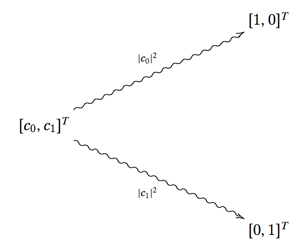
Observe that, before measuring it, any qubit can be written as a linear combination of classical bits:
\[\begin{bmatrix} c_0 \\ c_1 \end{bmatrix} = c_0 \cdot | \mathbf{0} \rangle + c_1 \cdot | \mathbf{1} \rangle\]Some examples are:
\[\begin{bmatrix} \tfrac{1}{\sqrt{2}} \\ \tfrac{1}{\sqrt{2}} \end{bmatrix} = \frac{1}{\sqrt{2}} \cdot | \mathbf{0} \rangle + \frac{1}{\sqrt{2}} \cdot | \mathbf{1} \rangle = \frac{| \mathbf{0} \rangle + | \mathbf{1} \rangle}{\sqrt{2}}\]and
\[\begin{bmatrix} \tfrac{1}{\sqrt{2}} \\ -\tfrac{1}{\sqrt{2}} \end{bmatrix} = \frac{1}{\sqrt{2}} \cdot | \mathbf{0} \rangle - \frac{1}{\sqrt{2}} \cdot | \mathbf{1} \rangle = \frac{| \mathbf{0} \rangle - | \mathbf{1} \rangle}{\sqrt{2}}\]How are qubits to be implemented? Think of electrons in different orbits, photons in one of two polarized states, particles in one of two spin directions.
What if we have many qubits? We define multi-particle qubits as:
\[|\mathbf{0} \rangle \otimes | \mathbf{1} \rangle \otimes \cdots \otimes |\mathbf{1} \rangle\]Since each state is described by two complex numbers $c_i$, the total number numbers required to describe a $n$-qubit system is $\mathbb{C}^{2^n}$. There are different ways to denote multiparticle qubits; here, we will stick to $|\mathbf{0} \mathbf{1} \cdots \mathbf{1} \rangle$.
Classical gates
We will not delve into the details of classical gates; we assume that the reader can have a look of definitions of classical gates here. What we will discuss is the ability to represent the action of a gate on a classical state as a matrix-vector multiplication over the binary field.
For example: consider the NOT gate. I.e., the input is a single classical bit; the output is its inverse. Using our notation, let us use as input $| \mathbf{0} \rangle$. Then, the NOT gate can be represented as:
\[\underbrace{\begin{bmatrix} 0 & 1 \\ 1 & 0 \end{bmatrix}}_{\text{NOT gate}} \cdot | \mathbf{0} \rangle = \begin{bmatrix} 0 & 1 \\ 1 & 0 \end{bmatrix} \cdot \begin{bmatrix} 0 \\ 1 \end{bmatrix} = \begin{bmatrix} 1 \\ 0 \end{bmatrix} = | \mathbf{1} \rangle\]Similar logic applies for other gates such as AND, NOR, XOR, NAND. In all cases, we can represent the application of the gate on an input as a matrix-vector product. For the gates with input more than a single bit, we can represent the input as the vertical concatenation of bits. Finally, when we have more than one gate in sequence, we can represent the sequence of matrices as a sequence of matrix-matrix multiplications, before we apply the input. Also, gates in parallel can be represented as kronecker products of matrices.
As an example consider the following sequence of gates:
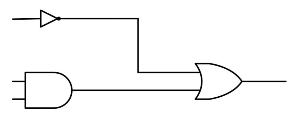
This can be described as OR(NOT, AND). Let us first compute the parallel set of gates NOT and AND.
\[\text(NOT) \otimes \text{AND} = \begin{bmatrix} 0 & 1 \\ 1 & 0 \end{bmatrix} \otimes \begin{bmatrix} 1 & 1 & 1 & 0 \\ 0 & 0 & 0 & 1 \end{bmatrix} = \begin{bmatrix} 0 & 0 & 0 & 0 & 1 & 1 & 1 & 0 \\ 0 & 0 & 0 & 0 & 0 & 0 & 0 & 1 \\ 1 & 1 & 1 & 0 & 0 & 0 & 0 & 0 \\ 0 & 0 & 0 & 1 & 0 & 0 & 0 & 0 \end{bmatrix}\]Also, combining the gates in sequence:
\[\text{OR(NOT, AND)} = \text{OR} \cdot (\text{NOT} \otimes \text{AND}) = \begin{bmatrix} 0 & 0 & 0 & 0 & 1 & 1 & 1 & 0 \\ 1 & 1 & 1 & 0 & 0 & 0 & 0 & 1 \end{bmatrix}\]You can verify that this matrix actually corresponds to the gate OR(NOT, AND).
Reversible classical (and quantum) gates
As we have seen so far, working in quantum systems provides also the notion of time that can move forward or backwards. I.e., we can apply unitary matrices that transform the current state, but also apply its inverse and go back to the initial state.
We can easily observe that not all classical gates can be applied in the quantum world, exactly due to this ineffiency to get back to the initial state. E.g., the AND gate with output 0 gives no information about which of the two input bits were 0 or whether both of them were 0.
In contast, there are classical gates that are reversible. E.g., the NOT gate. We can say that the NOT gate preserves the input information (=energy) while the AND gates fail to preserve the input information (=energy).
Note: an interesting topic to read is that of Landauer’s principle. We will skip this in this post.
Here, we will describe some gates that are both used in classical and quantum computing; purely quantum gates will be described later on.
A universal gate is a gate that can implement any Boolean function, without the need of any other gates. In classical computing, NAND and NOR are universal gates; fun fact is that AND and OR gates are constructed as NAND and NOR gates, followed but an inverter.
Controlled-NOT gate
The controlled-NOT gate takes two inputs and gives back two outputs. The schematic representation of it is as follows:
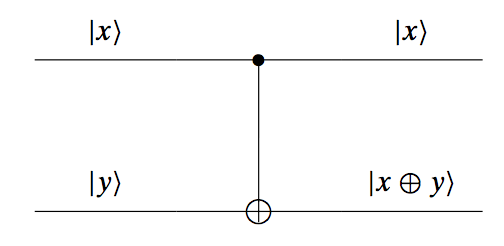
This gate operates as follows: the top input goes through the gate as it is, and we observe it at the output. However, the top signal controls the bottom signal: if the top signal is $|0\rangle$, then the input $|y\rangle$ will be output as it is; if the top signal is $|1\rangle$, then the gate reverses the bottom signal. We can see that the operation on the bottom signal is similar to an XOR gate, that’s why we use the symbol $\bigoplus$.
Toffoli gate
The Toffoli gate is similar to the controlled-NOT gate, but has three input signals, two of which “decide” about the output of the last input. Its schema is as follows:
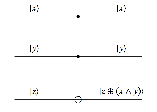
Here, the bottom signal flips only if both the top two inputs are equal to $|1\rangle$. The Toffoli gate is a universal gate (it is interesting to show by yourself that Toffoli can generate both the AND and the OR gate, from which one implies that it can generate the NAND gate, which by itself is known to be an universal gate).
Fredkin gate
Another universal gate is the Fredkin gate. Similar to the Toffoli gate, this gate has three inputs and three outputs:
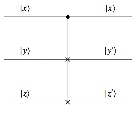
Only the top input operates as a controller: if it is $|0\rangle$, then the other two inputs output their values as they are; if it is $|1\rangle$, then the outputs of the two other signals are switched: we see $|y’\rangle = |z\rangle$ and $|z’\rangle = |y\rangle$. The Fredkin gate is also an universal gate.
Quantum gates
What we have talked so far is about gates that apply abstractly on both classical bits and quantum qubits. Here, we will discuss about gates that have a meaning when applied only on qubits.
Three key gates-matrices, widely used in quantum computing, are the Pauli matrices:
\[X \equiv \sigma_x = \begin{bmatrix} 0 & 1 \\ 1 & 0 \end{bmatrix}, ~~ Y \equiv \sigma_y = \begin{bmatrix} 0 & -j \\ j & 0 \end{bmatrix}, ~~ Z \equiv \sigma_z = \begin{bmatrix} 1 & 0 \\ 0 & -1 \end{bmatrix}.\]Each Pauli matrix is a hermitian matrix (we will see that all quantum gates are represented as hermitian and unitary, for energy preservation), and together with the identity matrix form a basis for the space of $2 \times 2$ Hermitian matrices.
Some other important quantum gates are:
- the S-gate: $S = \begin{bmatrix} 1 & 0 \ 0 & e^{j\pi/2} \end{bmatrix}$,
- the Hadamard gate: $H = \tfrac{1}{\sqrt{2}}\begin{bmatrix} 1 & 1 \ 1 & -1 \end{bmatrix}$,
- the T-gate: $T = \begin{bmatrix} 1 & 0 \ 0 & e^{\pi/4} \end{bmatrix}$.
All the above gates can be easily extracted from the generator matrix $U_3(\theta, \phi, \lambda)$, where:
\[U_3(\theta, \phi, \lambda) = \begin{bmatrix} \cos(\theta/2) & -e^{j\lambda} \sin(\theta/2) \\ e^{j\phi}\sin(\theta/2) & e^{j(\phi + \lambda)} cos(\theta/2) \end{bmatrix}\]Then, the Hadamard matrix is $H = U_3(\pi/2, 0, \pi)$, $S = U_3(0, 0, \pi/2)$, and $T = U_3(0, 0, \pi/4)$.
All the above operations are connected through the following properties:
- $X^2 = Y^2 = Z^2 = I$,
- $H = \tfrac{1}{\sqrt{2}} \left(X + Z\right)$,
- $X = HZH$,
- $Z = HXZ$,
- $S = T^2$.
Some other gates are the square root of NOT gate and the measurement gate, which is actually not reversible (and thus not unitary). The measurement gate is used usually at the end of quantum computations in order to obtain the answer from qubits (into bits).