Introduction to quantum computing: Grover’s algorithm.

Sources:

“Quantum computing for computer scientists”, N. Yanofsky and M. Mannucci, Cambridge Press, 2008.

This is part of a (probably) long list of posts regarding quantum computing.

In the last post, we discussed about Deutsch’s algorithm (and some of its variations). In this post, we will focus on a more known algorithm, that of Grover. Overall, Grover’s algorithm is a quadratic acceleration, over classical methods, for item search tasks in database applications (assuming databases are based or using a quantum computer - again this reminds me the dragon recipe…).

The overall task is as follows: given a list of items, find the requested item in time less than that required by exhaustive search.

Disclaimer I: while the material below might seem too simple for some scientists, I suggest not skimming over this post - personally, I always enjoy reading something that I believe I own, as επαναληψη μητηρ πασης μαθησεως (repetition is the mother of any knowledge)

The problem setting

In math terms, given a set a set of $n$ elements, how do you find a specific element in this set? The standard way to do so is through exhaustive search: we look into each individual entries in the list and report the solution when we find that particular entry. This could happen at the very beginning of the list (if we are extremelly lucky) or at the very end of the list (if we are extremelly unlucky). Overall, since algorithmic complexity has to do with Big-Oh notation and worst case scenaria, exhaustive search has $O(n)$ computational complexity.

Can we do better? Grover’s algorithm claims to solve the problem with high probability in $O(\sqrt{n}$) time. Be aware of the “high probability” statement, since the algorithm is not deterministic.

The way we are going to encode the problem is as follows. Assume we are given a function $f:{0, 1}^n \rightarrow {0, 1}$ that satisfies:

I.e., we are looking for the binary number $\mathbf{x}_0$ among all different $2^n$ possible numbers. The naive approach would be to check all $2^n$ instances of $\mathbf{x}$ and find when $f(\mathbf{x}) = 1$.

Two key ingredients

We will now describe two key ingredients that will help us achieve our goals. These are phase inversion and inversion about the mean. At first sight, these might be irrelevant to the problem we discuss, but their combination is crucial for Grover’s algorithm.

Phase inversion

The main idea behind the phase inversion is to change the phase of the (complex) weight/probability that corresponds to the element $\mathbf{x}_0 \in {0, 1}^n$. Let’s make this a bit more clear with an example: consider the simple case of $n=2$. I.e., we have 4 different numbers ${00, 01, 10, 11}$ and w.l.o.g. we assume that $\mathbf{x}_0 = 10$.

Design the following circuit:

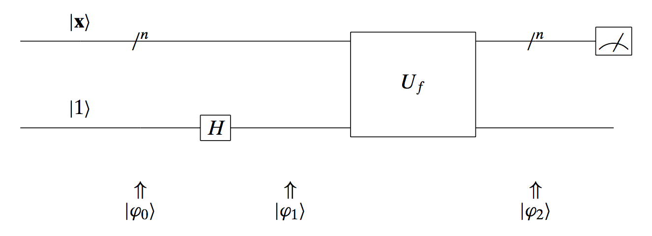
What can we achieve with this circuit? The top input is the $\mathbf{x}$ vector that we want to check whether it is the one we are looking for. The bottom input is a single qubit that is transformed by a Hadamard transform. The final outcome of the whole circuit satisfies:

What’s the idea behind this operation? Assume we start with a set of weights/probabilities in the case of fully superpositioned $|\mathbf{x}\rangle$: $\left[\tfrac{1}{2}, ~\tfrac{1}{2}, ~\tfrac{1}{2}, ~\tfrac{1}{2}\right]^{\top}$. Remember that we take the amplitudes squared to compute the probabilities. After using above circuit, we get the weight/probability vector: $\left[\tfrac{1}{2}, ~\tfrac{1}{2}, ~-\tfrac{1}{2}, ~\tfrac{1}{2}\right]^{\top}$. I.e., we changed the phase of the entry corresponding to the desired number $10$. Nevertheless, the probability of observing $10$ if we measure $\mathbf{x}$ at the end of the circuit is still $1/4$: $\left|-\tfrac{1}{2}\right|^2 = \tfrac{1}{4}$.

This is seemingly… useless, but in combination with the following ingredient, it can be really powerful.

Inversion about the mean

Let us now consider the second ingredient. We will use the example, described in the book “Quantum computing for computer scientists”, N. Yanofsky and M. Mannucci, Cambridge Press, 2008. Consider a given sequence of numbers: $X ={53, 38, 17, 23, 79}$. The average of this sequence is: $\bar{X} = 42$. The inversion about the mean is exactly what it implies: we are asked to find a different sequence of numbers such that $(i)$ the new numbers (summed up together) have the same distance as before from the mean, but inverted around the mean, $(ii)$ The new sequence has the same mean. As can be easily proved, the second part is automatically proven if the first part is true.

For example, for the first number in $X$, the distance from the mean $\bar{X}$ is $53 - \bar{X} = 11$. Thus, the number that has the same distance from the mean but inverted is: $-53 + 2\bar{X} = -53 + 2\cdot 42 = 31$. Similarly, we can see that the same rule:

applies for all cases and results into a new sequence: $\widehat{X} = {31, 46, 67, 61, 5}$. Observe that this sequence has the same mean as before, and all numbers are the mirrored versions around the mean of the initial sequence.

Applying phase inversion and inversion about the mean, sequentially

Let us consider an example. We will apply these two steps sequentially and focus on the fourth element of the vector.

We start with a vector X = [10, 10, 10, 10, 10], whose mean is 10. The difference 
between the fourth element and the rest is: 0.
1. Phase inversion: [10, 10, 10, -10, 10]. 
2. Mean inversion: The mean now is X_bar = 6. The rule for mean inversion is: 
-X_i + 2X_bar. Thus, we get: [2, 2, 2, 22, 2]. The difference between the fourth
element and the rest is: 20 - it increased!
3. Phase inversion: [2, 2, 2, -22, 2]. 
4. Mean inversion: The mean now is X_bar = -2.8. Then, we get: 
[-7.6, -7.6, -7.6, 16.4, -7.6,]. The difference between the fourth element 
and the rest is: 24 - it increased!
...

We can easily observe that the combination of phase and mean inversion in sequence stretches the distance between the entry of interest and the rest of the entries in the vector. I.e., in a way we force the element of interest to stand out compared to the rest of the entries.

Phase and mean inversion as quantum gates

So far, we described these two key ingredients in settings not so close to quantum computing. Let’s see how we can represent them in our setting. Remember that in the initial definition of the function $f$, we take as input binary strings with length $n$ and we output a binary number, with 1 only in the case where the input sequence matches the numer we look for.

One way to represent the phase and mean inversions together is as follows:

where $A = \tfrac{1}{2^n} \cdot \mathbb{1}_{2^n \times 2^n}$ is the matrix with all entries equal to $\tfrac{1}{2^n}$.

So, what is this matrix? First of all, $A$ matrix is the matrix that computes the mean. For example, in the case of 5 elements $v = [53, 38, 17, 23, 79]^\top$, and $A = \tfrac{1}{5} \cdot \mathbb{1}_{5 \times 5}$, we have:

I.e., the result computes the mean in each entry.

If on top of that we compute the full expression, we get: $(-I + 2A) v = [31, 46, 67, 61, 5]^\top$. I.e., we perform phase and mean inversion with this expression. One can also easily proof that the transformation $(-I + 2A)$, is actually unitary; thus we have hopes to implement it as a quantum gate.

Putting all the ingredients together: The Grover’s algorithm

Grover’s algorithm can be described with a quantum circuit as follows:

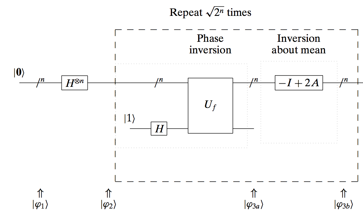
The algorithm performs the following motions:

• Set top input to $|\mathbf{0}\rangle$
• Apply the Hadamard transform to put in superposition all possible outcomes, with equal probability.
• Repeat $\sqrt{2^n}$ times:
  • Apply phase inversion
  • Apply mean inversion about the mean
• Measure output - with high probability, the result will be the entry required.

To show the power of Grover’s algorithm, we will close our post with an example. We consider $n = 3$. The possible states are: [“000”, “001”, “010”, “011”, “100”, “101”, “110”, “111”]. Our function $f$ is equal to one only at the state “101”. Following the algorithm above we have:

• Initially: $|\mathbf{\varphi}_1 \rangle = [0 ~0 ~0 ~0 ~0 ~0 ~0 ~0]^\top$.
• After applying the Hadamard transfrom, we get: $|\mathbf{\varphi}_2 \rangle = \left[\tfrac{1}{\sqrt{8}} ~\tfrac{1}{\sqrt{8}} ~\tfrac{1}{\sqrt{8}} ~\tfrac{1}{\sqrt{8}} ~\tfrac{1}{\sqrt{8}} ~\tfrac{1}{\sqrt{8}} ~\tfrac{1}{\sqrt{8}} ~\tfrac{1}{\sqrt{8}}\right]^\top$.
• In the inner loop:
  • The phase inversion gives: $|\mathbf{\varphi}_{3a} \rangle = \left[\tfrac{1}{\sqrt{8}} ~\tfrac{1}{\sqrt{8}} ~\tfrac{1}{\sqrt{8}} ~\tfrac{1}{\sqrt{8}} ~\tfrac{1}{\sqrt{8}} ~-\tfrac{1}{\sqrt{8}} ~\tfrac{1}{\sqrt{8}} ~\tfrac{1}{\sqrt{8}}\right]^\top$.
  • The mean of the vector of probabilities is: $\frac{7\cdot \tfrac{1}{\sqrt{8}} -\tfrac{1}{\sqrt{8}}}{\sqrt{8}} = \frac{3}{4 \sqrt{8}}$.
  • After inversion around the mean, our vector of probabilities becomes: $|\mathbf{\varphi}_{3b} \rangle = \left[\tfrac{1}{2\sqrt{8}} ~\tfrac{1}{2\sqrt{8}} ~\tfrac{1}{2\sqrt{8}} ~\tfrac{1}{2\sqrt{8}} ~\tfrac{1}{2\sqrt{8}} ~\tfrac{5}{2\sqrt{8}} ~\tfrac{1}{2\sqrt{8}} ~\tfrac{1}{2\sqrt{8}}\right]^\top$.
  • … (after one more iteration in the inner loop).
• Measuring the top output, we get: $|\mathbf{\varphi}_{3b} \rangle = \left[-\tfrac{1}{4\sqrt{8}} ~-\tfrac{1}{4\sqrt{8}} ~-\tfrac{1}{4\sqrt{8}} ~-\tfrac{1}{4\sqrt{8}} ~-\tfrac{1}{4\sqrt{8}} ~\tfrac{11}{4\sqrt{8}} ~-\tfrac{1}{4\sqrt{8}} ~-\tfrac{1}{4\sqrt{8}}\right]^\top$.

Observe that the probability to measure “101” is: $|\tfrac{11}{4\sqrt{8}}|^2 = 0.9453125$, while any other entry appears in the output with probability: $|\tfrac{11}{4\sqrt{8}}|^2 = 0.0078125$. Thus, even with two iterations, we get the solution we want with probability getting pretty close to 1!