In this notebook, $(i)$ we will further dive in the original IHT scheme and note some of its pros/cons in solving the CS problem, and $(ii)$ we will provide an overview of more recent developments on constant step size selection for IHT.

To connect with the previous post, we have briefly discussed the importance of CS via an image compression/de-compression application (there are several more!) and, we have formulated the classic CS problem via a non-convex optimization problem criterion.

A closer look into the IHT algorithm

Recall the IHT iteration, \(\mathbf{x}_{i+1} = \mathcal{H}_{k} \left(\mathbf{x}_{i} + \boldsymbol{\Phi}^\top \cdot (\mathbf{y} - \boldsymbol{\Phi} \mathbf{x}_i)\right).\) We remind that $\mathcal{H}_{k}(\cdot)$ is the hard thresholding operator that keeps the $k$ largest in magnitude elements of the input vector.

Again, according to this post, IHT is nothing else than projected gradient descent in a non-convex setting: \(\mathbf{x}_{i+1} = \mathcal{H}_{k} \left(\mathbf{x}_{i} - \mu \nabla f(\mathbf{x}_i)\right)\) where $\nabla f(\mathbf{x}_i) := -\boldsymbol{\Phi}^\top \cdot (\mathbf{y} - \boldsymbol{\Phi} \mathbf{x}_i)$ and the step size is set to $\mu = 1$.

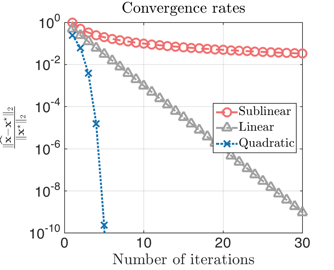
Convergence rate. According to the two theorems in this post, IHT shows linear convergence. Those of you that know what linear convergence means, just skip the following comments and continue with the next paragraph. For the rest of us, this note succinctly describes the differences in convergence rates: sublinear, linear, superlinear, etc. As a rule of thumb, just remember that the descrease in distance $||\widehat{\mathbf{x}} - \mathbf{x}^\star||_2$ (in logarithmic scale):

• … finds a ‘plateau’, as the iterations increase, in the sublinear rate case.
• … decreases as a linear function in the linear rate case.
• … decreases as a “minus quadratic” function in the quadratic rate case.

For a visual interpretation, see the next plot:

To make a comparison with convex methods, linear convergence rate is the best one can hope for, by only using first-order (gradient) information [1]. To this end, IHT could be considered optimal, in a convergence rate sense.

Computational complexity. It is obvious that IHT has low-computational complexity per iteration. The bottleneck lies in the gradient calculation: $\nabla f(\mathbf{x}_i) := -\boldsymbol{\Phi}^\top \cdot (\mathbf{y} - \boldsymbol{\Phi} \mathbf{x}_i)$, which depends on matrix-vector multiplications. These can be computed in $O(n p)$ time. The hard-thresholding operator $\mathcal{H}_{k}(\cdot)$ requires $O(p \log p)$ complexity due to sorting. (N.B.: Seeing IHT as a solver for generic $f$, the computational bottleneck depends on the ‘complexity’ of the objective function and how easy it is to compute its gradient; see [2] for a generalization of IHT to more generic problems.)

Ease of implementation. Not many things to say here: IHT is easy to implement!

Step size selection. In general, using a constant and – more importantly – independent-to-the-problem step size (as is the case here, $\mu = 1$) might effect the efficiency of the algorithm, under various problem settings. What we mean by that? Let us consider the following example.

%matplotlib inline
import numpy as np
import scipy as sp
import math
import matplotlib.pyplot as plt
from bokeh.plotting import figure, show, output_file
from bokeh.palettes import brewer

from mpl_toolkits.mplot3d import Axes3D
import matplotlib.cm as cm

import random
from numpy import linalg as la

p = 1000  # Ambient dimension
n = 300   # Number of samples
k = 100   # Sparsity level

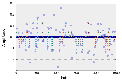
# Generate a p-dimensional zero vector
x_star = np.zeros(p)
# Randomly sample k indices in the range [1:p]
x_star_ind = random.sample(range(p),  k) 
# Set x_star_ind with k random elements from Gaussian distribution
x_star[x_star_ind] = np.random.randn(k)
# Normalize
x_star = (1 / la.norm(x_star, 2)) * x_star

# Plot
plt.style.use('bmh')
xs = range(p)
markerline, stemlines, baseline = plt.stem(xs, x_star, '-.')
plt.setp(markerline, 'alpha', 0.3, 'ms', 6)
plt.setp(markerline, 'markerfacecolor', 'b')
plt.setp(baseline, 'color', 'r', 'linewidth', 1, 'alpha', 0.3)
plt.xlabel('Index')
plt.ylabel('Amplitude')
plt.show()

# Generate sensing matrix
Phi = (1 / math.sqrt(n)) * np.random.randn(n, p)

# Observation model
y = Phi @ x_star

Let us run again IHT algorithm (for completeness, we copy the code here).

# Hard thresholding function
def hardThreshold(x, k):
    p = x.shape[0]
    t = np.sort(np.abs(x))[::-1]    
    threshold = t[k-1]
    j = (np.abs(x) < threshold)
    x[j] = 0
    return x

# Returns the value of the objecive function
def f(y, A, x):
    return 0.5 * math.pow(la.norm(y - Phi @ x, 2), 2)

def IHT(y, A, k, iters, epsilon, verbose, x_star):
    # Length of original signal
    p = A.shape[1]
    # Length of measurement vector
    n = A.shape[0]
    # Initial estimate
    x_new = np.zeros(p)    
    # Transpose of A
    At = np.transpose(A)

    # Initialize
    x_new = np.zeros(p)           # The algorithm starts at x = 0

    PhiT = np.transpose(Phi)
    
    x_list, f_list = [1], [f(y, Phi, x_new)]

    for i in range(iters):
        x_old = x_new
    
        # Compute gradient
        grad = -PhiT @ (y - Phi @ x_new)
    
        # Perform gradient step
        x_temp = x_old - grad    
    
        # Perform hard thresholding step
        x_new = hardThreshold(x_temp, k)
    
        if (la.norm(x_new - x_old, 2) / la.norm(x_new, 2)) < epsilon:
            break
                
        # Keep track of solutions and objective values
        x_list.append(la.norm(x_new - x_star, 2))
        f_list.append(f(y, Phi, x_new))
        
        if verbose:
            print("iter# = "+ str(i) + ", ||x_new - x_old||_2 = " + str(la.norm(x_new - x_old, 2)))
    
    print("Number of steps:", len(f_list))
    return x_new, x_list, f_list
        
# Run algorithm
epsilon = 1e-6                # Precision parameter
iters = 20

x_IHT, x_list, f_list = IHT(y, Phi, k, iters, epsilon, True, x_star)

# Plot
plt.rc('text', usetex=True)
plt.rc('font', family='serif')

xs = range(len(x_list))
plt.plot(xs, x_list, '-o', color = '#3399FF', linewidth = 4, alpha = 0.7, markerfacecolor = 'b')
plt.yscale('log')
plt.xlabel(r'\text{Iterations}')
plt.ylabel(r"$\|\mathbf{x}^\star - \widehat{\mathbf{x}}\|_2$")

# Make room for the ridiculously large title.
plt.subplots_adjust(top=0.8)
plt.show()

iter# = 0, ||x_new - x_old||_2 = 1.59899422893
iter# = 1, ||x_new - x_old||_2 = 3.25412215459
iter# = 2, ||x_new - x_old||_2 = 9.06574106157
iter# = 3, ||x_new - x_old||_2 = 25.4511255305
iter# = 4, ||x_new - x_old||_2 = 75.2643807267
iter# = 5, ||x_new - x_old||_2 = 231.196758137
iter# = 6, ||x_new - x_old||_2 = 727.337120296
iter# = 7, ||x_new - x_old||_2 = 2322.74281939
iter# = 8, ||x_new - x_old||_2 = 7457.43786837
iter# = 9, ||x_new - x_old||_2 = 24163.2629567
iter# = 10, ||x_new - x_old||_2 = 78812.8454198
iter# = 11, ||x_new - x_old||_2 = 258976.23671
iter# = 12, ||x_new - x_old||_2 = 852391.100305
iter# = 13, ||x_new - x_old||_2 = 2816600.59026
iter# = 14, ||x_new - x_old||_2 = 9338169.18343
iter# = 15, ||x_new - x_old||_2 = 31098623.121
iter# = 16, ||x_new - x_old||_2 = 103362897.097
iter# = 17, ||x_new - x_old||_2 = 344580080.476
iter# = 18, ||x_new - x_old||_2 = 1149967576.66
iter# = 19, ||x_new - x_old||_2 = 3844704422.82
Number of steps: 21

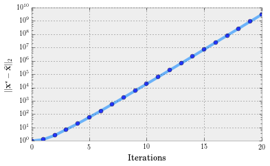
It diverges! The only difference of this setting, compared to the previous post, is the sparsity level: here, it is $k = 100$, while in our initial illustration it was $k = 10$. The rest of the parameters (ambient dimension $p$ and number of measurements $n$) remain the same. Why does this make a difference?

The purpose of this post is to highlight the importance of step size selections in such iterative schemes. As it will be apparent next (and more clearly in the next post), one of the reasons for this poor performance of IHT is its simplistic step size selection procedure.

But first, to answer these questions, let us introduce the notion of phase transition in CS problems.

Phase transition in CS problems

We will describe the notion of phase transition for the convex $\ell_1$-norm minimization case (explicit phase transitions for non-convex case have not been proved yet – in case I’m wrong, I would love to discuss it with you!): \(\min_{\mathbf{x}} \|\mathbf{x}\|_1 \quad \text{s.t.} \quad \mathbf{y} = \boldsymbol{\Phi} \mathbf{x}.\) In their seminal work [3-4], Tanner and Donoho explicitly characterize the performance of such $\ell_1$-norm minimization criterion, using the notion of phase transition. We quote (and rephrase) from [5]:

In the case of $\ell_1$-norm minimization with $\boldsymbol{\Phi}$ a random sensing matrix, there is a well-defined “break-point”: even given infinite computational power, there are problem configurations (sparsity vs. ambient dimension vs. number of samples) where the above criterion fails to find the ground truth. On the other hand, such optimization criterion can successfully recover the sparsest solution, provided that sparsity level $k$ is smaller than a certain definite fraction of ambient dimension $p$.

The above introduce the following figure into our discussion (N.B.: see this site).

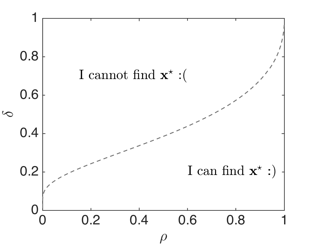
Here, $\delta := \frac{n}{p}$ is a normalized measure of problem indeterminacy, i.e., how much information we have in terms of linear observations w.r.t. ambient dimension. Also, $\rho = \frac{k}{n}$ denotes a normalized measure of the sparsity; e.g., observe that one needs $n = k + 1$ to find a $k$-sparse signal. Then, (and I quote again [5]) the above figure describes the difficulty of a problem instance: problems are intrincically harder as one moves up and the left. Also, points in the figure indicate success and failure as a function of position in phase space.

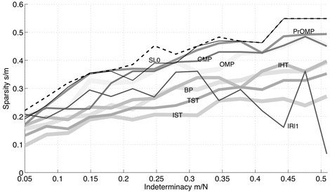
The above are the conclusion of a rigorously proven theorem that describes asymptotic properties of the $\ell_1$-norm criterion. For any other algorithm, there is only emprirical evidence; see the following plot from this site – BP is the $\ell_1$-norm criterion.

What’s the bottomline? It might be the case that IHT, with step size $\mu = 1$, fails to solve this problem just because it is out of its capabilities, with high probability! In the next post, we will describe specific techniques that lead to adaptive step size selections and solve problem instances that vanilla IHT cannot.

For completeness, we present next several attempts on finding a different constant step size selection. This discussion will be also helpful for our next post. The crux is that, even if more sophisticated constant step size selections lead to better theoretical guarantees, it usually is the case that computing such step size is as hard as the initial problem!

GraDeS (or IHT with a different constant step size)

At the same time IHT was published, Garg and Khandekar [6] proposed GraDeS, an IHT variant with constant step size selection. Actually, the only difference between IHT and GraDeS is that the latter uses step size $\mu = \frac{1}{1 + \delta_{2k}}$, instead of $\mu = 1$. This leads to the following guarantees:

Theorem 1 (Convergence of IHT in function values) [7]. Suppose $\mathbf{x}^\star$ is an $k$-sparse vector satisfying $\mathbf{y} = \boldsymbol{\Phi} \mathbf{x}^\star$ and the isometry constants of the matrix $\boldsymbol{\Phi}$ satisfies $\delta_{2k} < 1/3$. Then, IHT computes an s-sparse vector $\widehat{\mathbf{x}} \in \mathbb{R}^p$ such that $||\mathbf{y} - \boldsymbol{\Phi} \widehat{\mathbf{x}}||_2 \leq \epsilon$ in \(\Bigg\lceil \frac{1}{\log\left(\tfrac{1 − \delta\_{2k}}{2\cdot \delta\_{2k}}\right)} \cdot \log \left(\frac{\|\|\mathbf{y}\|\|\_2 ^2}{\epsilon}\right) \Bigg\rceil\) iterations.

In other words, GraDeS converges linearly to the optimal solution (as IHT does) and requires a less strict condition on the RIP constants of the sensing matrix ($\delta_{2k} < 1/3$ vs. $\delta_{3k} < 1/15$).

This is great news! So, what is left is to compute the RIP constant of $\boldsymbol{\Phi}$ and use it for step size in IHT. But how can we compute (or at least approximate) $\delta_{2k}$? It turns out that, given sensing matrix $\boldsymbol{\Phi}$, computing its RIP constants is…(wait for it!) at least as hard as the original combinatorial problem! (N.B.: In [6], GraDeS is implemented with a constant step size – in particular $\mu = 1/3$ and $\mu = 3/4$).

Why $\mu = \frac{1}{1 + \delta_{2k}}$? Just to provide some intuition about GraDeS step size selection, we make the connection with that made in convex optimization.

Consider the following convex optimization problem: \(\min_{\mathbf{x}} f(\mathbf{x})\) where $f(\mathbf{x})$ satisfies Lipschitz gradient continuity with constant $L > 0$ (otherwise stated, $f$ is smooth - however, $f$ being smooth is a much stricter assumption – see here):

for any $\mathbf{x}_1,~\mathbf{x}_2$ in the domain of $f$. “Optimal” first-order (gradient) methods by Nesterov [1] suggest the following recursion: \(\mathbf{x}_{i+1} = \mathbf{x}_i - \mu \cdot \nabla f(\mathbf{x}_i)\) where the step size is set to $\mu = \frac{1}{L}$. It turns out that such constant step size selection is sufficient to provide attractive convergence guarantees for any $f$.

Let us compute Lipschitz constant in CS problem. Focusing on $k$-sparse vectors $\mathbf{x}_1,~\mathbf{x}_2$, we compute:

where $(i)$ $\mathcal{S}$ denotes the union of non-zero indices in $\mathbf{x}_1,~\mathbf{x}_2$ – observe that $|\mathcal{S}| \leq 2k$, $(ii)$ here $\mathcal{S}$ denotes the placeholder for any possible, at most $2k$-sparse combination of sparsity supports, $(iii)$ is due to RIP; see also [7, Section 5.1].

In other words, convex optimization wisdom suggests step size $\mu = \frac{1}{1 + \delta_{2k}}$!

Constant step size selection for non-symmetric RIP matrices

In one of my first research attempts during my PhD [8], Volkan and I provide a another constant step size selection. To be even more generic, we consider the case of non-symmetric RIP matrices:

Definition (Non-symmetric Restricted Isometry Property - RIP). An $n \times p$ matrix $\boldsymbol{\Phi}$ satisfies the non-symmetric restricted isometry property for sparsity level $k \geq 1$ if there exist constans $\alpha_k, ~\beta_k$ such that the inequalities \(\alpha_k \|\mathbf{x}\|_2^2 \leq \|\boldsymbol{\Phi} \mathbf{x}\|_2^2 \leq \beta_k \|\mathbf{x}\|\_2^2\) hold for all $\mathbf{x} \in \mathbb{R}^p$ with $||\mathbf{x}||_0 \leq k$.

For our step size derivation, we use the convergence proof of IHT – in vector estimates, not in function values – where step size is considered as a variable. This note lists the basic steps that lead to the following recursive formula for IHT:

Here, $\mathcal{A} := \mathcal{S}^\star \cup \mathcal{S}_{i} \cup \mathcal{S}_{i+1}$. Observe that

To optimize the convergence rate, one can pick $ \mu $ as the minimizer of the expression: \(\min_{\mu} \|\mathbf{I} - \mu \boldsymbol{\Phi}_{\mathcal{A}}^\top \boldsymbol{\Phi}_{\mathcal{A}}\|_2 \leq \min_{\mu} \max \lbrace \mu \cdot \beta_{3k} - 1, 1 - \mu \cdot \alpha_{3k} \rbrace,\)

which leads to the following result, inspired by convex optimization constant step size strategies [1].

Lemma 1 (Non-symmetric RIP constant step size strategy) [8]. Assume $ \boldsymbol{\Phi} $ satisfies the non-symmetric RIP with known upper/lower bounds $ \alpha_{cK}, \beta_{cK}, (c = 2,3) $. The step size $ \mu $ that implies the fastest convergence rate in the recursion above amounts to \(\mu = \frac{2}{\alpha_{3k} + \beta_{3k}}.\)

In the special case where $ \boldsymbol{\Phi} $ satisfies the symmetric RIP for some constant $ \delta_{3k} $, we have:

Corollary 1 (RIP constant step size strategy) [8]. Given $ \boldsymbol{\Phi} $ satisfies the RIP for some $ \delta_{3k} $, the step size $ \mu $ that implies the fastest convergence rate in the above lemma amounts to $\mu = 1$. Moreover, this step size results in contraction (noiseless case): \(\|\mathbf{x}_{i+1} - \mathbf{x}^\star\|_2 \leq \rho \cdot \|\mathbf{x}_i - \mathbf{x}^\star\|_2\) with $ \rho = 2\delta_{3k} $. I.e., $ |\rho| < \frac{1}{2} $ implies that we require $\delta_{3k} < 1/4 $.

Connection with step size selection in convex settings. We note that, for strongly convex and Lipschitz gradient continuous functions, Nesterov again [1] suggests as step size: $\mu = \frac{2}{M + L}$, where $M$ is the strong convexity parameter and $L$ is the Lipschitz parameter. We remind that a strongly convex and Lipschitz gradient continuous function satisfies: \(M \mathbf{I} \preceq \nabla ^2 f(\mathbf{x}) \preceq L \mathbf{I}\) It is not hard to see that non-symmetric RIP (as well as classic RIP) implies similar spectral inequalities, restricted on the domain of sparse vectors: \(\alpha_k \mathbf{I} \preceq \nabla ^2 f(\mathbf{x}) \preceq \beta_k \mathbf{I}, ~ ~ ~ ~\forall k\text{-sparse vectors}.\) This is also related to the notion of restricted strong convexity and smoothness in [9-10].

Conclusion

It is obvious that computing such step sizes in practice is inefficient. That being said, in the next post:

• We will describe some adaptive step size strategies for IHT.
• We will start introducing the ALPS framework, that includes IHT as a special case.

A small note on RIP constants and convergence rate. As a concluding remark for this post, I would like to note the significance of RIP constants in the convergence proofs of such algorithms.

From an optimization point of view, improving the conditions on these constants might seem insignificant: IHT has already linear convergence and convex wisdom suggests that this is the best we could do.

From a signal processing point of view though, improving such conditions means that the algorithm succeeds under weaker assumptions: requiring $\delta_{ck} < \gamma$ where $c$ is as small as possible and $\gamma$ as big as possible implies that the algorithm will provably find the true $\mathbf{x}^\star$ under a wider set of design matrices. I.e., requiring $\delta_{ck} < \gamma$ for a very small $\gamma$ signifies that we need to try harder to design a proper matrix or we have less chances of succeding using a random selected sensing matrix.

On the other hand and as we will see in the next post, stricter conditions of the form $\delta_{ck} < \gamma$ do not necessarily indicate that the algorithm is actually worse in practice: as we make algorithms more sophisticated (by introducing more processing steps), we introduce more ‘places’ in our analysis which might lead to loose bounds in our theory.

Bottomline, things are not as simple as they seem!

References

[1] Yurii Nesterov, Introductory lectures on convex optimization, Vol. 87, Springer Science & Business Media, 2004.

[2] Sohail Bahmani, Raj Bhiksha and Petros T. Boufounos, Greedy sparsity-constrained optimization, The Journal of Machine Learning Research 14.1 (2013): 807-841.

[3] David Donoho and Jared Tanner, Neighborliness of randomly projected simplices in high dimensions, Proceedings of the National Academy of Sciences of the United States of America 102.27 (2005): 9452-9457.

[4] David Donoho and Jared Tanner, Counting faces of randomly projected polytopes when the projection radically lowers dimension, Journal of the American Mathematical Society 22.1 (2009): 1-53.

[5] Arian Maleki and David Donoho, Optimally tuned iterative reconstruction algorithms for compressed sensing, Selected Topics in Signal Processing, IEEE Journal of 4.2 (2010): 330-341.

[6] Rahul Garg, and Rohit Khandekar, Gradient descent with sparsification: An iterative algorithm for sparse recovery with restricted isometry property, in ICML, 2009.

[7] Deanna Needell and Joel Tropp, CoSaMP: iterative signal recovery from incomplete and inaccurate samples, Communications of the ACM 53.12 (2010): 93-100.

[8] Anastasios Kyrillidis, and Volkan Cevher, Recipes on hard thresholding methods, 4th IEEE International Workshop on Computational Advances in Multi-Sensor Adaptive Processing (CAMSAP), 2011.

[9] Alekh Agarwal, Sahand Negahban, and Martin Wainwright, Fast global convergence rates of gradient methods for high-dimensional statistical recovery, In Advances in Neural Information Processing Systems, pages 37–45, 2010.

[10] Sahand Negahban and Martin Wainwright, Restricted strong convexity and weighted matrix completion: Optimal bounds with noise, The Journal of Machine Learning Research, 13(1):1665– 1697, 2012.