The AdaDelta algorithm

In this short note, we will briefly describe the AdaDelta algorithm. AdaDelta belongs to the family of stochastic gradient descent algorithms, that provide adaptive techniques for hyperparameter tuning. The paper can be found here.

Disclaimer: These notes assume that the reader can build up the story by looking at the mathematical expressions. Also, please read the post on AdaGrad.

Problem setting

The problem setting is:

Like the motivation in AdaGrad, setting the learing rate properly typically involves tuning procedures in order to find the highest step size that leads to fast convergence, and avoids divergence.

AdaGrad alleviates this obstacle via a new dynamic learning rate that is computed per-dimension (i.e., each variable/parameter enjoys a different step size) and is based only on first-order information. However, Adagrad is sensitive to initial conditions: if the initial gradients are large, the learning rates will be low for the remainder of training. One way to lessen this problem is to tune the global learning rate $\eta$: however, this cancels the advantage of AdaGrad as being an adaptive learning rate algorithm.

The AdaDelta variation

Let us first define the following quantities:

with initial condition: $\mathbb{E}[g^2]_0 = 0$. For simplicity, assume we compute full gradients: i.e., $i_t$ contains all the indices of samples in the dataset. Here, $\left(\nabla f(x_t)\right)^2 \in \mathbb{R}^p$ and denotes the vector with entries the gradient entries, squared. This implies that $\mathbb{E}[g^2]_t$ is also a vector with the same dimensions. The term $\mathbb{E}[g^2]_t$ is the exponentially decaying average of squared gradients: in stark contrast to AdaGrad, we keep adding new information from squared gradients, but we also make sure to decrease the effect of old gradients.

The main iteration of AdaDelta, using only the above, is:

where $\text{RMS}[\cdot]$ denotes the root mean square metric.

Further, the main difference of AdaDelta to Adagrad is the hypothetical unit correction in the former. The idea is simply the following: While in Hessian methods the descent direction satisfies $H^{-1} \nabla f(x) \propto \text{units of } x$, in gradient methods, we have $\nabla f(x) \propto \tfrac{1}{\text{units of } x}$. Inspired by this observation, AdaDelta substitutes $\eta$ above with: \(\mathbb{E}[\Delta x^2]_t = \rho \mathbb{E}[\Delta x^2]_{t-1} + (1 - \rho) \Delta x_t^2\)

with initial condition: $\mathbb{E}[\Delta x^2]_0 = 0$. Then, AdaDelta becomes:

This concludes the main recursion of the AdaDelta algorithm.

Note: While AdaDelta is assumed to be parameter-free, there are some hyperparameters that need to be carefully tuned in order to exploit the most out of the algorithm. These parameters include $\rho$ in running averages and the $\varepsilon$ constant. However, we agree that mispecification of such hyperparameters is less sensitive to erroneous performance, compared to mispecificition of the learning rates.

Some experiments

We will build on the experiments from our last post, check the validity of the AdaDelta algorithm, and see whether it performs better/same/worse than the so-far list of algorithms.

Well-conditioned linear regression

Let us explain again the settings we will work on - skip this part if you have already read the previous post.

Let $x^\star$ be the unknown vector in $\mathbb{R}^p$, assuming $|| x^\star ||_2 = 1$. In standard linear regression, we observe $x^\star$ via the linear mapping:

where $A \in \mathbb{R}^{n \times p}$ is the set of features, and $w \in \mathbb{R}^n$ is an additive noise term. For simplicity we can assume that $w$ is i.i.d. according to a Gaussian distribution, with mean zero and standard deviation $\sigma$.

Given the above, the problem we want to solve is:

for $a_i^\top$ being the rows of the matrix $A$.

It is well known that a key component for characterizing the convergence of an algorithm on such problems is the condition number $\kappa(F)$ of the problem. By definition, the condition number is the ratio:

Here, $L$ is the Lipschitz gradient constant of $F$ and $\mu$ its strong convexity parameter (afterall, we are still in the convex world). The largest the condition number, the harder (=more number of iterations to get a specific error tolerance $||\widehat{x} - x^\star||^2 \leq \varepsilon$ ) the problem is. For the case of least squares, the condition number of the problem is proportional to the condition number of $A^\top A$:

The setting is given in the code below - it is written in Maltab (another deprecated choice but personally I believe Matlab is still at the top of the list for algorithmic protoyping…).

%% Problem setting

% Dimension
p = 50;								

% Number of measurements
n = 200;							

% Noise std
sigma = 1e-3;						

% This will vary below.
kappa = 10^2;						

log_smin = -1;
log_smax = log10(sqrt(kappa) * 10^log_smin);

% Measurement matrix
A = 1/sqrt(n) * randn(n, p); 		
[U, ~, V] = svd(A, 'econ');

% Force condition number be kappa
S = logspace(log_smin, log_smax, p);
S = S(end:-1:1);					

A = U * diag(S) * V';

% Ground truth
x_star = randn(p, 1);				
x_star = x_star./norm(x_star);

% Noise
w = randn(n, 1);					
w = sigma * w./norm(w); 

% Measurements in y
y = A*x_star + w;					

• AdaDelta vs. AdaGrad vs. plain Gradient Descent with step size $\tfrac{1}{L}$.

For gradient descent, we use the recursion:

and we compare it to:

where $\zeta$ is set to a small number (say, $10^{-10}$).

For AdaDelta, according to the source paper, there is no step size parameter to tune. The only two parameters are the $\varepsilon$ parameter (which we set equal to $\zeta$ above) and the running average parameter $\rho$, which we set to $\rho = 0.95$ according to the paper.

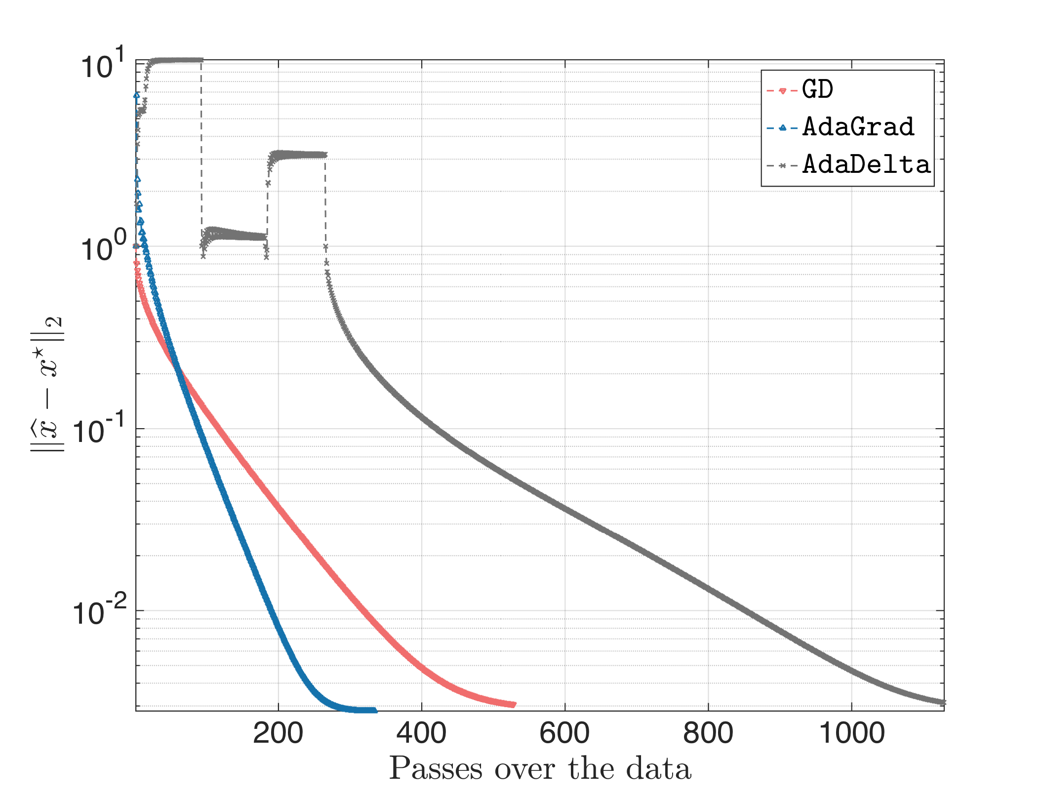
The result looks something like this:

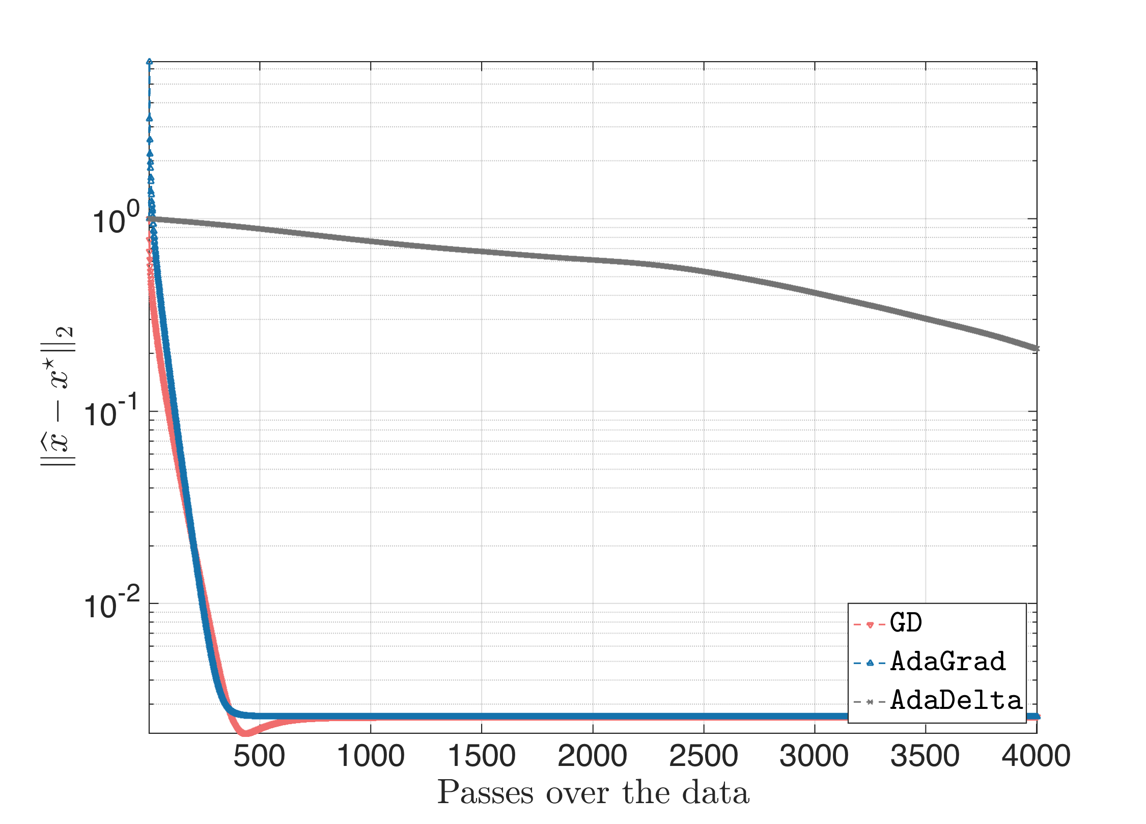
All algorithms start at the same all-zero starting point. While AdaGrad and GD perform similarly with fast convergence rate, AdaDelta has slow convergence and does not achieve a distance $|| \hat{x} - x^\star||_2$ less than $10^{-1}$. Inspecting the intermediate weights, for suggested initial conditions $\mathbb{E}[g^2]_0 = \mathbb{E}[\Delta x^2]_0 = 0$, we observed that often the gradient might have small (in magnitude) entries, and, thus, with a parameter $\rho$ close to one, forces the term $-\frac{\sqrt{\mathbb{E}[\Delta x^2]_t + \varepsilon}}{\sqrt{\mathbb{E}[g^2]_t + \varepsilon}} \odot \nabla f_{i_t}(x_{t})$ be small and with equal weights. This, in turn, makes $\mathbb{E}[\Delta x^2]_t$ not vary much, leading to overall slow convergence.

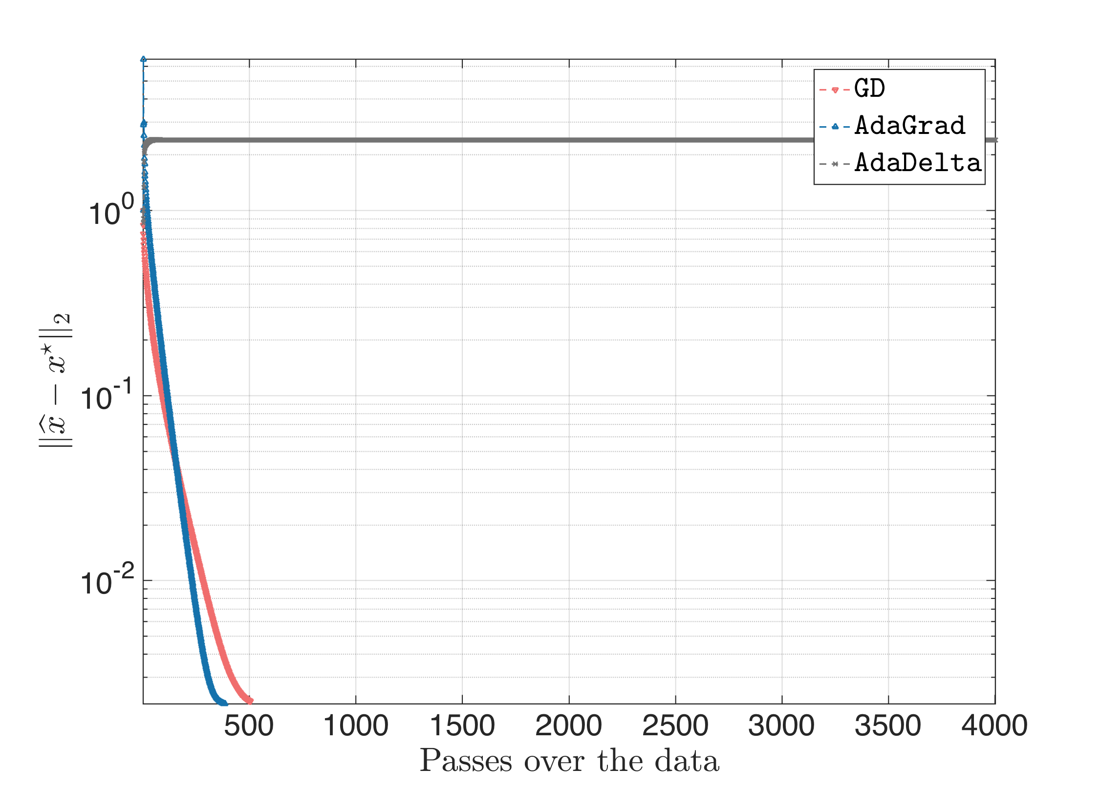
Actually, even if we set $\rho = 0$ (no running average), the result looks often like:

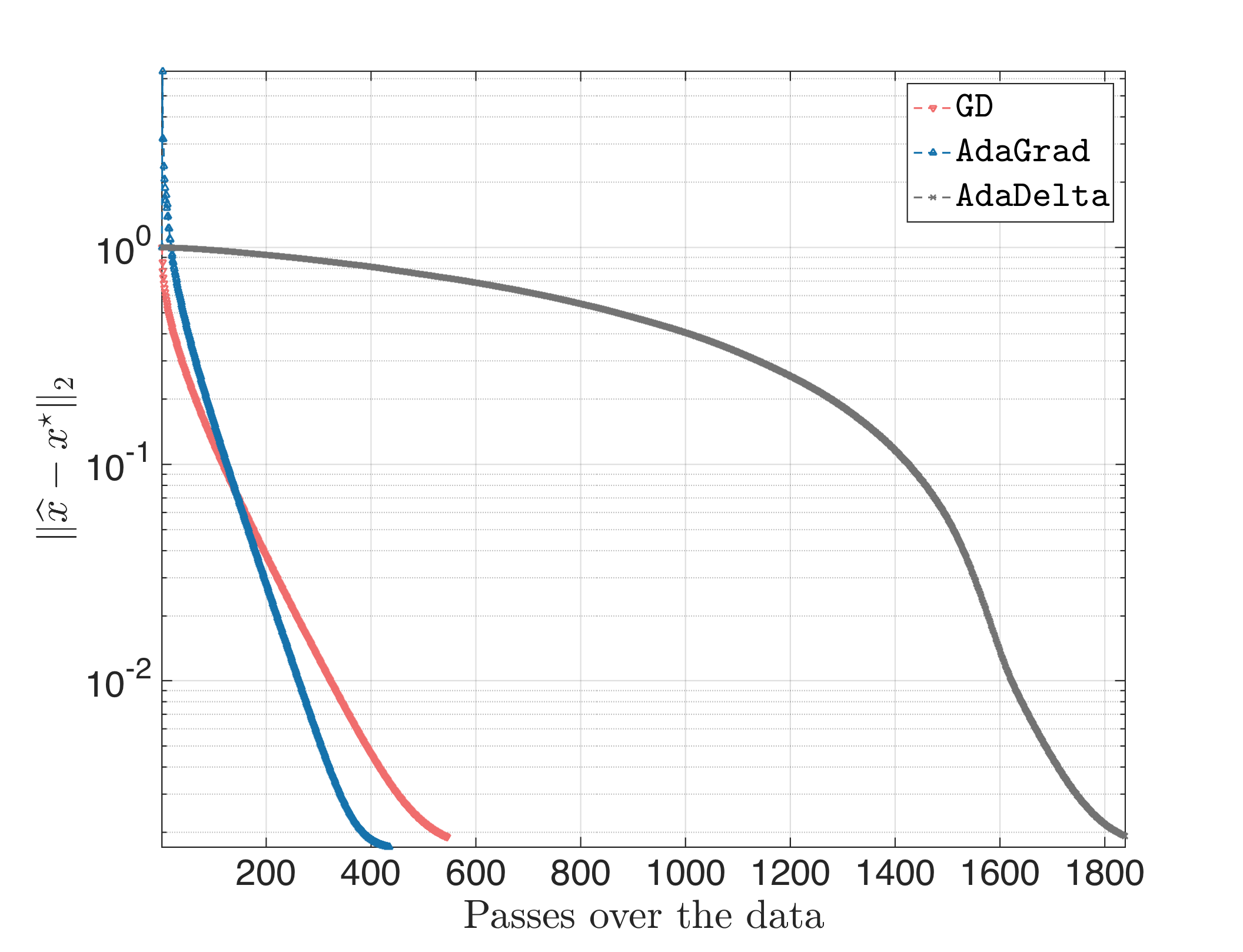
Let us try to modify AdaDelta a bit: it will be apparent that often “innocent” parameters or choices lead to tremendous differences. First, let’s see whether changing the current initialization $\mathbb{E}[g^2]_0 = \mathbb{E}[\Delta x^2]_0 = 0$ will change things: we force $\mathbb{E}[g^2]_0 \in [0, 1]^p $ and $\mathbb{E}[\Delta x^2]_0 \in [0, 1]^p$, randomly chosen. Fortunately, this might lead to (keeping $\rho = 0.95$):

but also to:

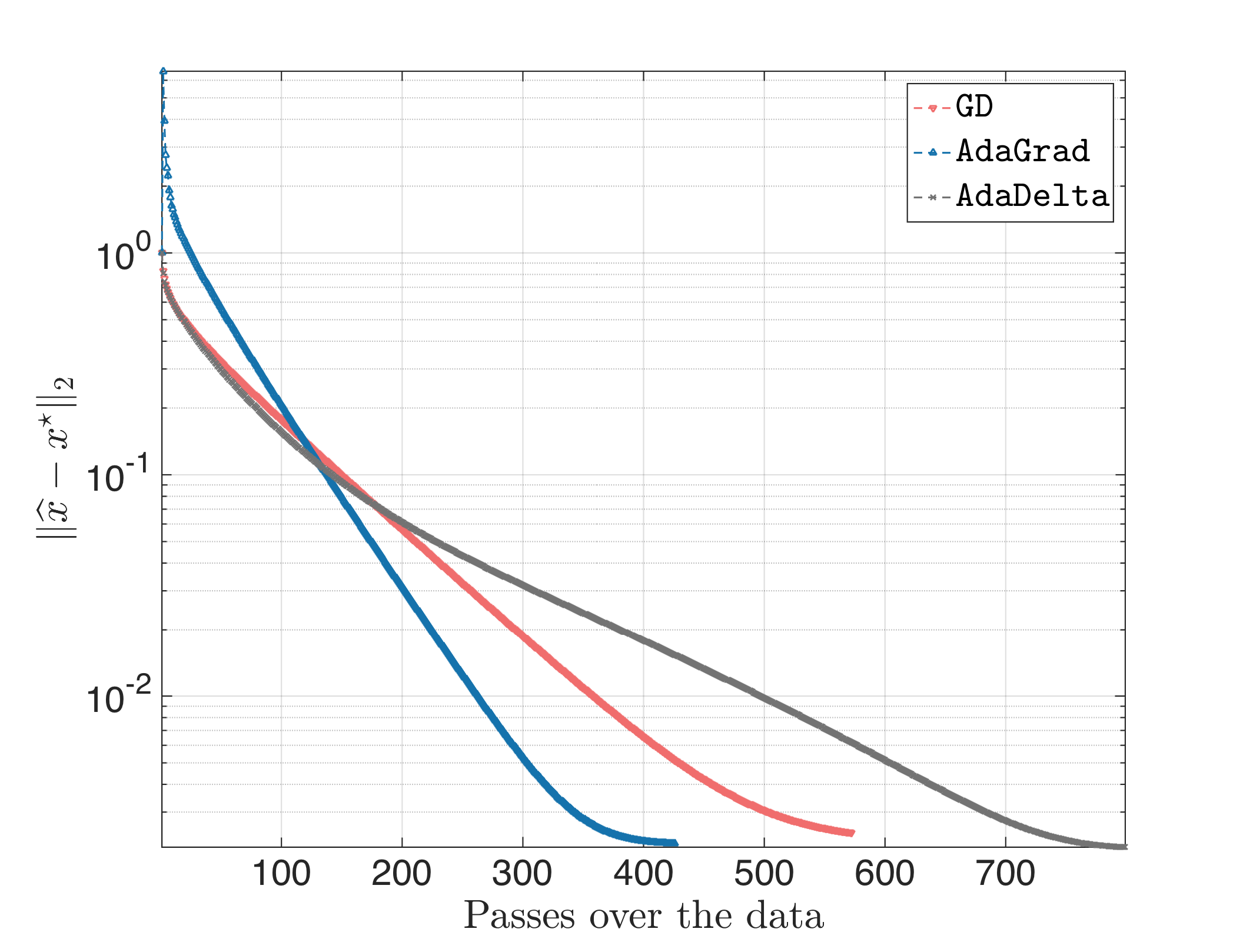
Since still $\mathbb{E}[g^2]_t$ and $\mathbb{E}[\Delta x_t^2]_t$ remain constant, we will make sure when this happens to restart the procedure. I.e., we check when the distances $|| \mathbb{E}[g^2]_t - \mathbb{E}[g^2]_{t-1}||_2$ or $|| \mathbb{E}[\Delta x_t^2]_t - \mathbb{E}[\Delta x_{t-1}^2]_{t-1} ||_2$ are small; in that case, we reset $\mathbb{E}[g^2]_0 \in [0, 1]^p $ and $\mathbb{E}[\Delta x^2]_0 \in [0, 1]^p$. We use as closeness parameter $10^{-3}$. In the worst case, the result looks like:

I.e., the algorithm had three failling initializations, while the last initialization led to faster convergence.

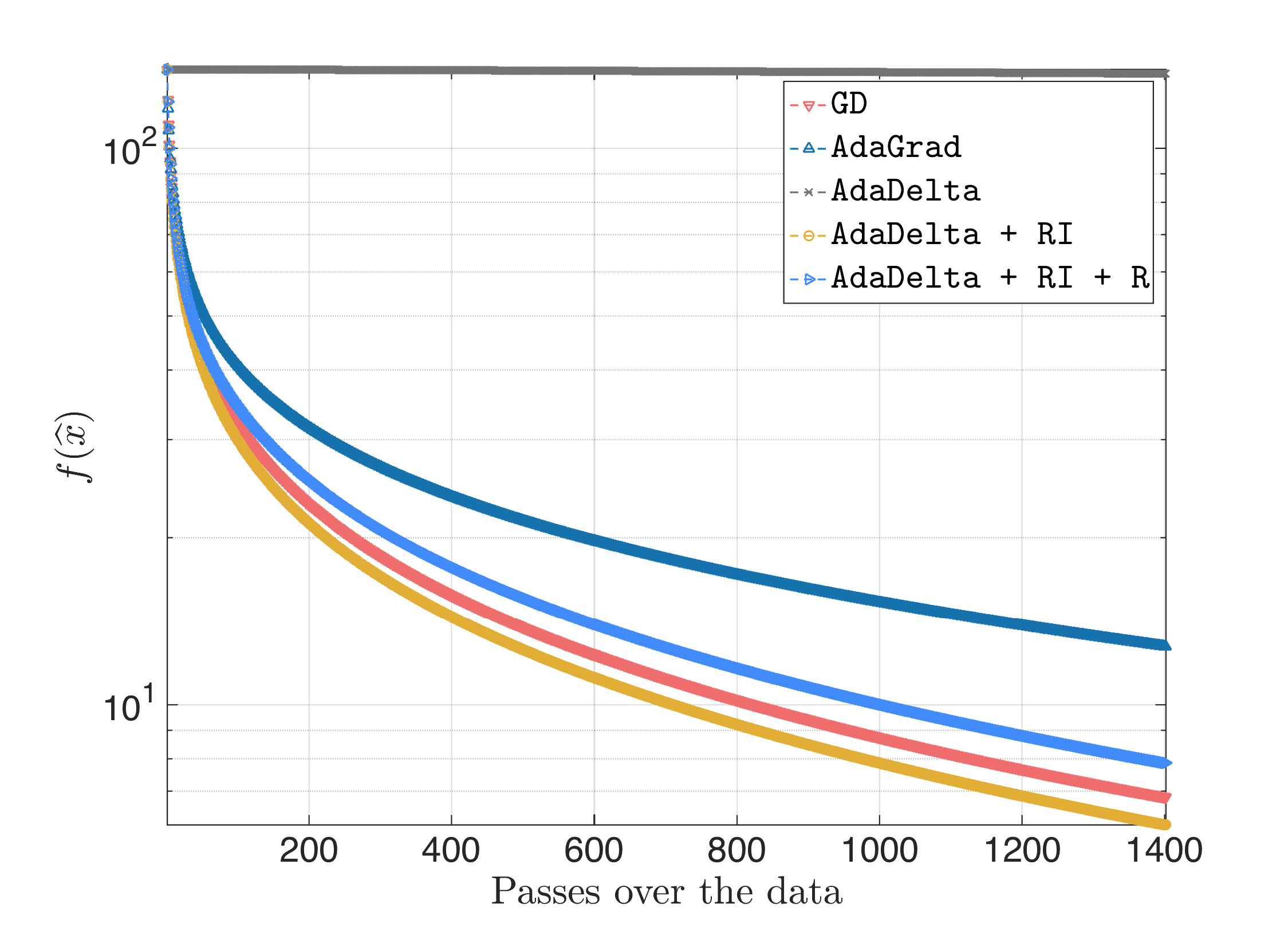
• AdaDelta vs. AdaGrad vs. plain Gradient Descent with step size $\eta = 0.1$.

Let us first rename AdaDelta with random initialization as $\texttt{AdaDelta + RI}$, and AdaDelta with random initialization and restart as $\texttt{AdaDelta + RI + R}$.

The result looks something like this:

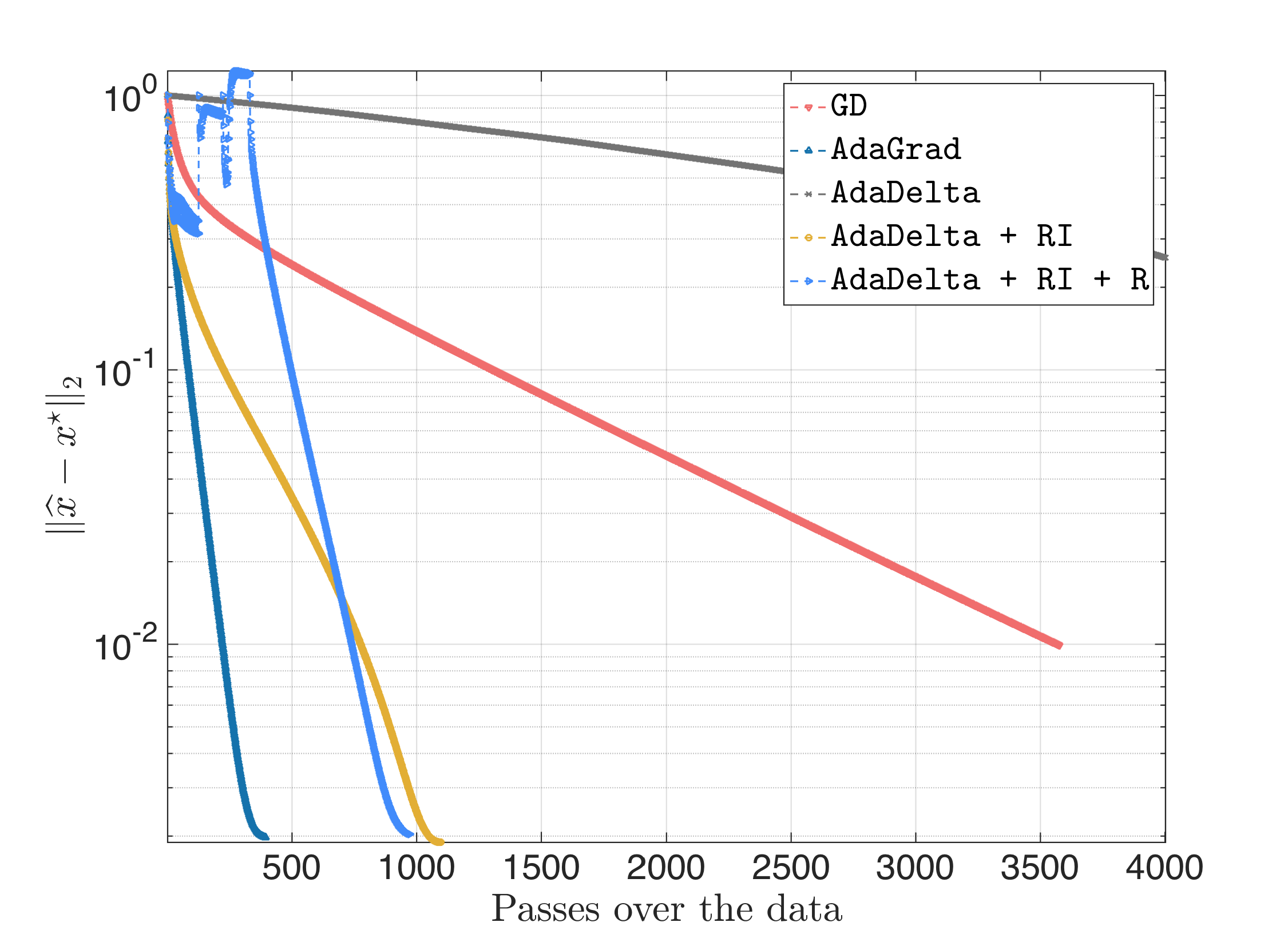
Remember, there are always runs of the code where $\texttt{AdaDelta + RI}$ does not converge.

• AdaDelta vs. AdaGrad vs. plain Gradient Descent with carefully selected step size.

From the discussion above, it is obvious that AdaDelta needs further tweak in order to achieve better performance (if possible), compared to GD or AdaGrad. Thus, we skip this step.

Ill-conditioned linear regression

Let us repeat the above experiment for $\kappa(A^\top A)$ much larger.

% New condition number
kappa = 10^6;						

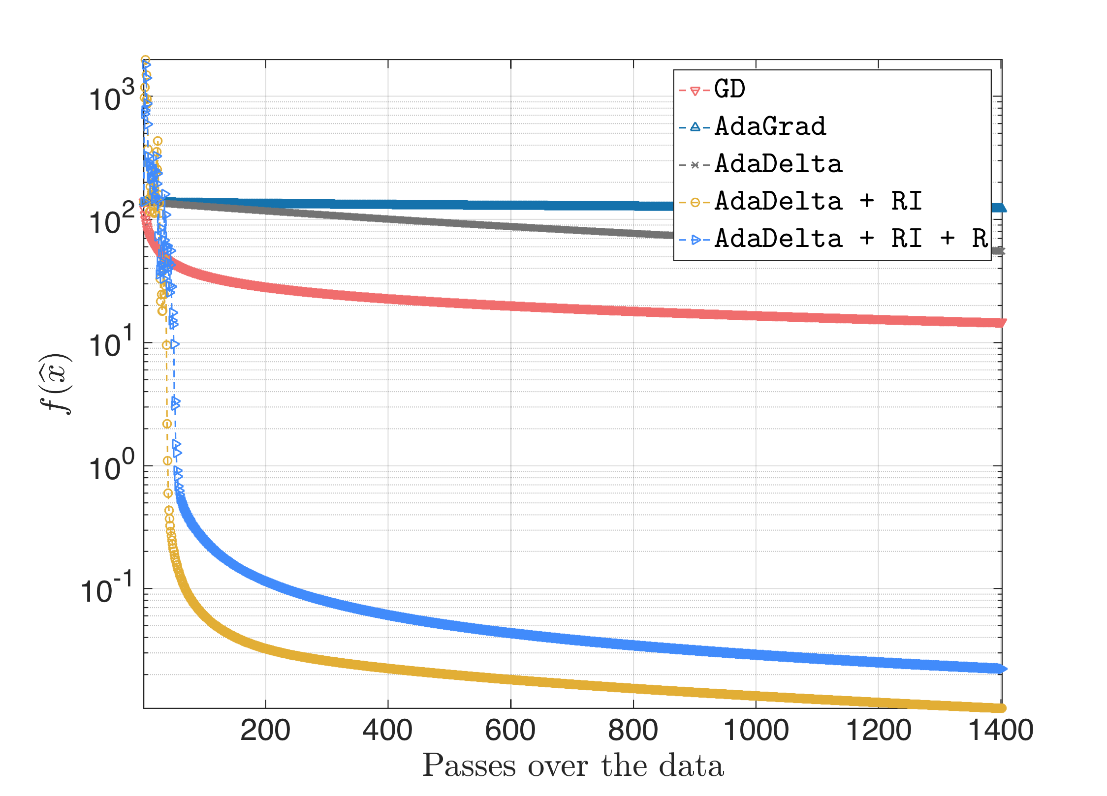
Following the same steps, for $\eta = \frac{1}{L}$ we get:

For $\eta = 0.1$, we get:

where Adagrad and AdaDelta still converge (with the latter being faster) and GD diverging.

Overall, for ill-conditioned problems, random initialization and restarts were unnecessary (actually, initialization as proposed in the source paper performs much better).

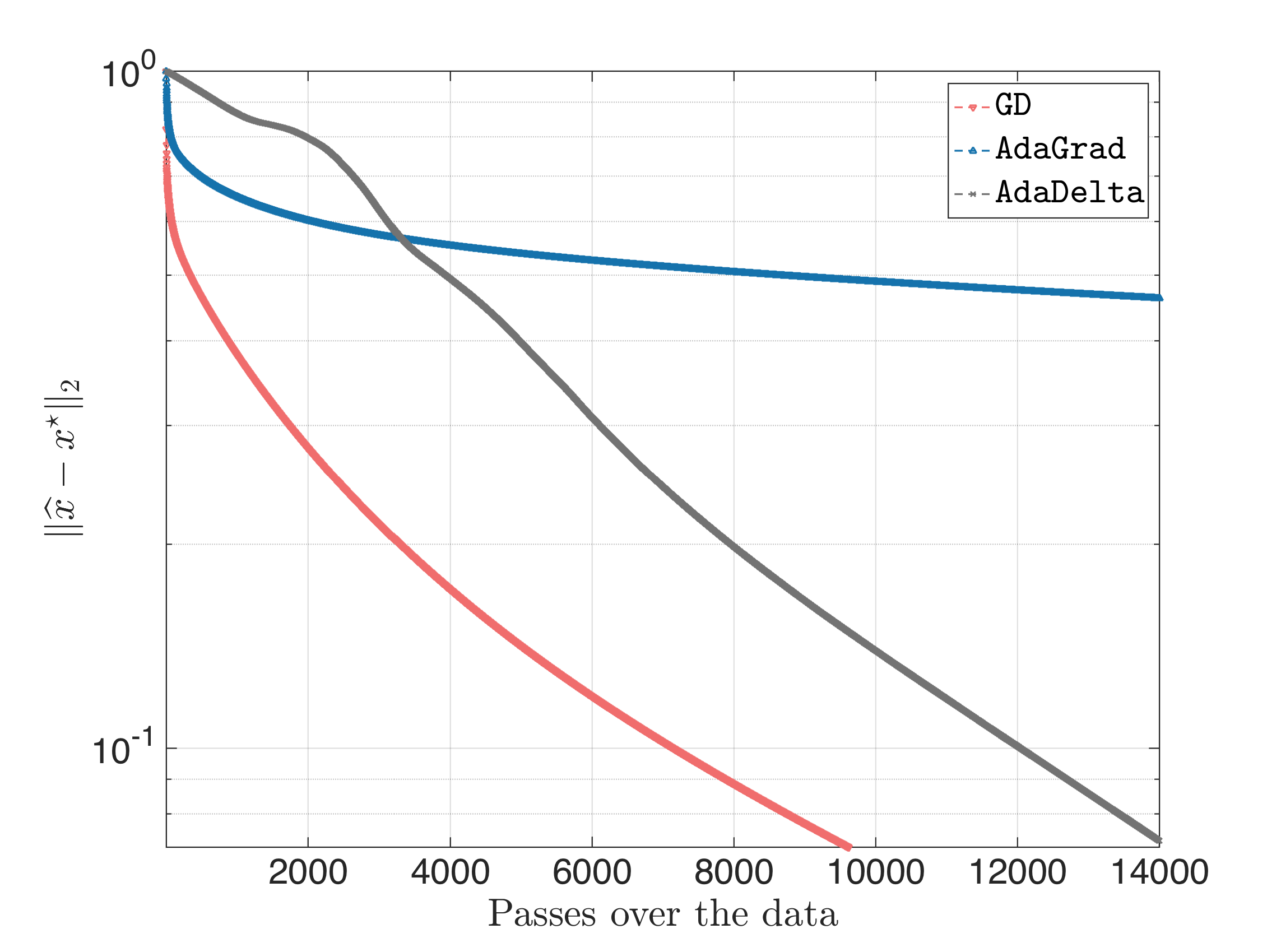
Logistic regression

Almost similar behavior was observed for the case of logistic regression. Let us assume for all cases that the step size for GD and AdaGrad is $\frac{1}{L}$. For condition number of the measurement matric $\kappa = 10^2$, we get:

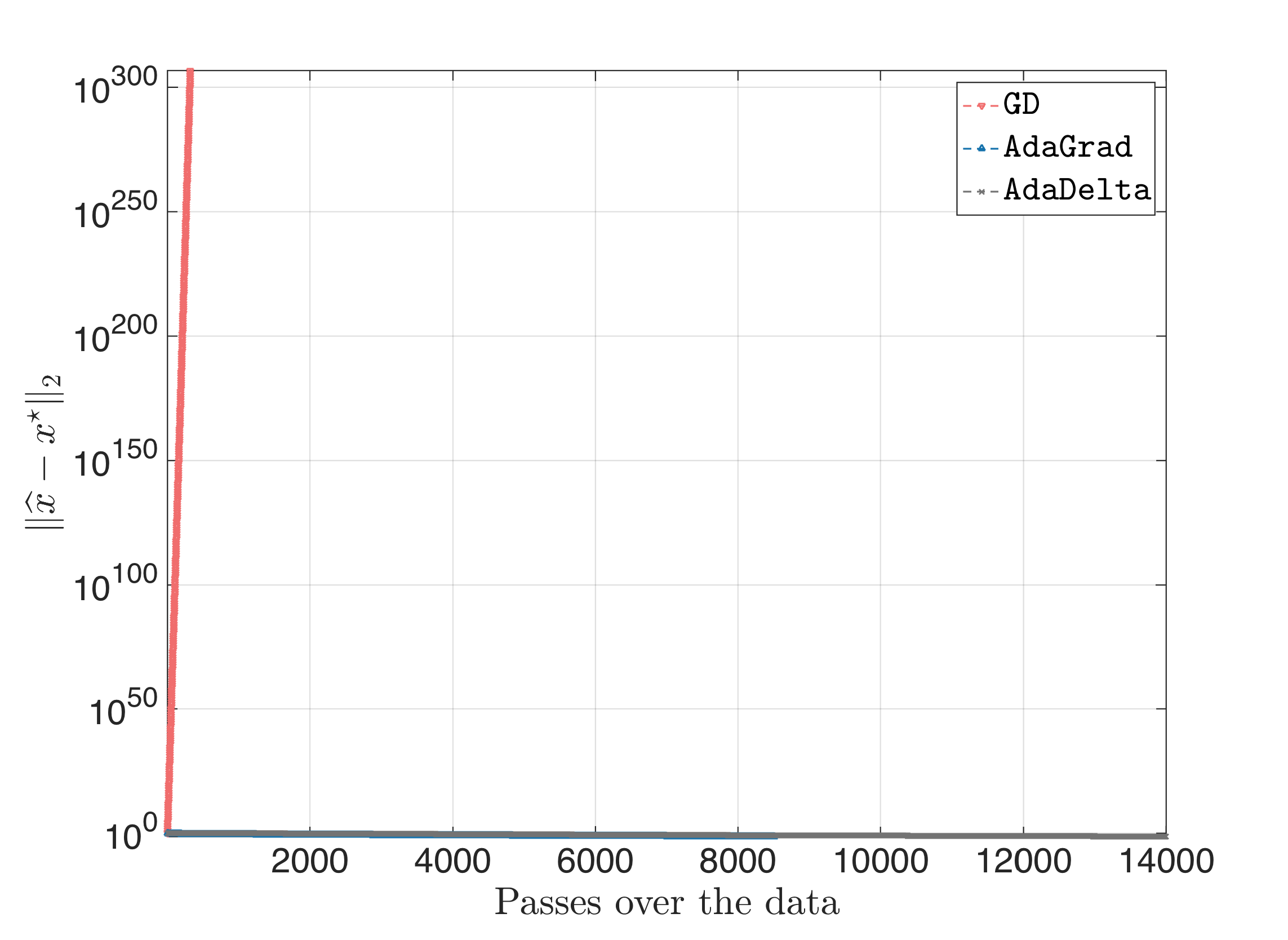
The surprising behavior is for ill-conditioned where $\kappa = 10^6$. We observe:

Feedforward Neural Network (FNN) training

To be written…